
Research
State Space Models, Explained Through Code
Written by

Karthik Ragunath Ananda Kumar
Choose how you want to experience Tavus. Whether you’re building with our APIs or meeting a PAL, you can switch anytime.
Build real-time, human-like AI experiences using Tavus APIs and tools.
Best for developers, founders, and teams integrating Tavus into a product.
Meet your personal AI companions who listen, remember, and are always present.
Best for individuals looking to talk, explore, and connect with a friend.
Written by
Karthik Ragunath Ananda Kumar
publish date
June 8, 2026
I built a minimal state space model in pure PyTorch and trained it character-by-character on tiny-shakespeare dataset to understand how SSMs and Mamba actually work. This post walks through that code and explains what each piece does, why it’s there, and how it all fits together.
A language model takes a sequence of tokens and predicts the next one. Transformers do this with attention: every new token looks at every previous token via \(\text{softmax}(QK^T)V\), which costs \(O(N^2)\) for training and forces you to keep every previous K and V in memory during inference.
State Space Models (SSMs) take a different route. Instead of letting each token see every previous token directly, they compress the entire past into a small fixed-size hidden state and update that state one token at a time. Cost per token: \(O(1)\). Memory: the hidden state, period. No cache that grows linearly with context.
Pure SSMs (S4, S5, H3) had this nice cost structure but couldn’t quite match transformer quality at scale. The reason was that their dynamics were “linear time-invariant”: the same recurrence applied to every token regardless of what the token was.
Take the recurrence \(h_t = \bar{A} h_{t-1} + \bar{B} x_t\) with fixed \(\bar{A} = 0.5\) and \(\bar{B} = 1\). Three inputs arrive: \(x_1 = 10\), \(x_2 = 6\), \(x_3 = 4\).
But look at where each piece of \(h_3\) actually came from:
| Original input | How old is it? | How many times halved? | Contribution to \(h_3\) |
|---|---|---|---|
| \(x_1 = 10\) | 2 steps ago | \(0.5^2 = 0.25\) | \(0.25 \times 10 = 2.5\) |
| \(x_2 = 6\) | 1 step ago | \(0.5^1 = 0.5\) | \(0.5 \times 6 = 3.0\) |
| \(x_3 = 4\) | just arrived | \(0.5^0 = 1\) | \(1 \times 4 = 4.0\) |
| total | \(2.5 + 3.0 + 4.0 = 9.5\) |
Every past input’s contribution follows the same rule: an input that arrived \(k\) steps ago has been multiplied by \(\bar{A}\) exactly \(k\) times. Its weight is \(\bar{A}^k \bar{B}\), regardless of what step we’re at. This weight schedule is the same everywhere in the sequence. It doesn’t matter if we’re computing \(h_5\) or \(h_{500}\). “Two steps ago” always means “multiplied by \(\bar{A}\) twice,” because \(\bar{A}\) is constant.
That’s basically a convolution: a fixed set of weights \((1.0, 0.5, 0.25, 0.125, \ldots)\) applied at every position. At position \(t\) the output is \(y_t = 1.0 \cdot x_t + 0.5 \cdot x_{t-1} + 0.25 \cdot x_{t-2} + \ldots\). Convolutions can be computed all at once (in parallel, or via FFT) without stepping through the sequence one position at a time. That’s the huge speed advantage of LTI: you never actually run the recurrence during training.
The problem is quality. The system can’t say “this is a content word, absorb it strongly” or “this is filler, ignore it.” Every token gets the same \(\bar{A}\) and the same \(\bar{B}\). It can’t selectively gate.
Mamba is the version that fixes this by letting the recurrence’s parameters depend on the current input, so each token can decide how much state to keep and how much new information to absorb. This “selectivity” is what closes most of the quality gap to attention while keeping the recurrent cost structure. The tradeoff: once \(\bar{A}\) and \(\bar{B}\) vary per token, the convolution trick breaks (the weight on “3 steps ago” now depends on which intervening tokens appeared), so you need either a sequential loop or a parallel scan to compute the recurrence. That’s why our implementation uses a plain for t in range(L) loop, and why the official Mamba code needs hand-tuned CUDA kernels.
The minimal model we’ll build has 4 Mamba blocks, d_model=128 (each token is represented as a 128-dimensional vector throughout the network), d_state=16 (the SSM carries 16 memory dimensions, each forgetting at a different rate, so some capture relationships between nearby tokens while others retain information from much earlier in the sequence). It trains on character-level tinyshakespeare dataset (65-token vocab -> {a - z, A - Z, !, ’, ,, -, ., :, ;, ?, &, $, 3, , and a space}, context window of 256) for 40000 steps and learns to generate Shakespeare-ish text.
Where SSMs show up in practice? The constant per-token cost and fixed-size state make SSMs especially attractive for real-time and streaming applications. Many production grade Text-to-speech systems use SSM backbones because they need to produce audio tokens at a steady rate without the growing latency of attention. Speech recognition, music generation, and video modeling benefit for the same reason: the sequence is long and you want constant-time generation per step.
Tinyshakespeare is ~1.1 MB of Shakespeare’s plays as one text file (downloaded on first run if not present locally). The vocabulary is built by collecting every unique character: 26 lowercase, 26 uppercase, digits, punctuation, space, newline. That gives 65 tokens total. stoi maps character to integer id, itos goes the other way:
chars = sorted(list(set(text)))
vocab_size = len(chars)   # 65
stoi = {c: i for i, c in enumerate(chars)}
itos = {i: c for i, c in enumerate(chars)}
The entire file is converted to a tensor of integer ids and split 90/10 into train/val:
data = torch.tensor([stoi[c] for c in text], dtype=torch.long)
n_train = int(0.9 * len(data))
train_data = data[:n_train]
val_data = data[n_train:]
Training works on fixed-length windows of block_size = 256 characters. The full training set is ~1 million characters, but we never feed it all at once. Each step, get_batch picks 64 random starting positions anywhere in the corpus and cuts out a 256-character window from each. Over thousands of steps, these overlapping windows cover the entire text many times, but no single forward pass ever processes more than 256 characters. Relationships between characters farther apart than 256 positions are invisible to the model during training.
At inference, though, we can generate text longer than 256 characters. The SSM’s hidden state h acts as a rolling summary of everything it has seen so far. When we generate token by token, each new token updates h, and the previous information doesn’t disappear just because we’ve passed position 256. The 256-character limit only applies to training (we can’t backpropagate gradients across a longer window), but at generation time the hidden state carries forward indefinitely. Whether the model actually remembers something from 500 tokens ago depends on how well it learned to use its state, but architecturally nothing stops it. In practice, since the model never saw dependencies longer than 256 during training, coherence degrades past that horizon.
def get_batch(split: str):
    d = train_data if split == "train" else val_data
    ix = torch.randint(0, len(d) - block_size - 1, (batch_size,))
    x = torch.stack([d[i : i + block_size] for i in ix])           # [B, L]
    y = torch.stack([d[i + 1 : i + 1 + block_size] for i in ix])   # [B, L]
    return x.to(device), y.to(device)
The key detail is that y is x shifted by one position. If x[b, t] is the character at position \(t\) in batch element \(b\), then y[b, t] is the character at position \(t+1\). That’s the next-token prediction setup: at position \(t\), the model sees x[b, t] (and everything before it) and must predict y[b, t] = x[b, t+1].
A toy example. Suppose block_size=5 and the underlying text is Hello, world!. One sampled window might be:
| position | 0 | 1 | 2 | 3 | 4 |
|---|---|---|---|---|---|
x (input) | H | e | l | l | o |
y (target) | e | l | l | o | , |
But the model doesn’t see each character in isolation. At each position, the SSM’s hidden state carries information from all previous characters. So what the model actually works with is the accumulated context:
| position | context seen | must predict |
|---|---|---|
| 0 | H | e |
| 1 | He | l |
| 2 | Hel | l |
| 3 | Hell | o |
| 4 | Hello | , |
At position 0 the model sees only H and must predict e. At position 4 it has seen Hello and must predict ,. Every position is a training example, so a single forward pass produces 256 predictions in parallel. Over 5000 iterations with batch 64, we sample ~80 million character positions from a 1 million character file, so every character gets visited many times, each time with a different preceding context.
Before we get to Mamba’s code, we need to understand the mathematical object it’s built on: a state space model. Start with the simplest possible version, a single scalar input feeding a hidden state of size \(N\), producing a scalar output.
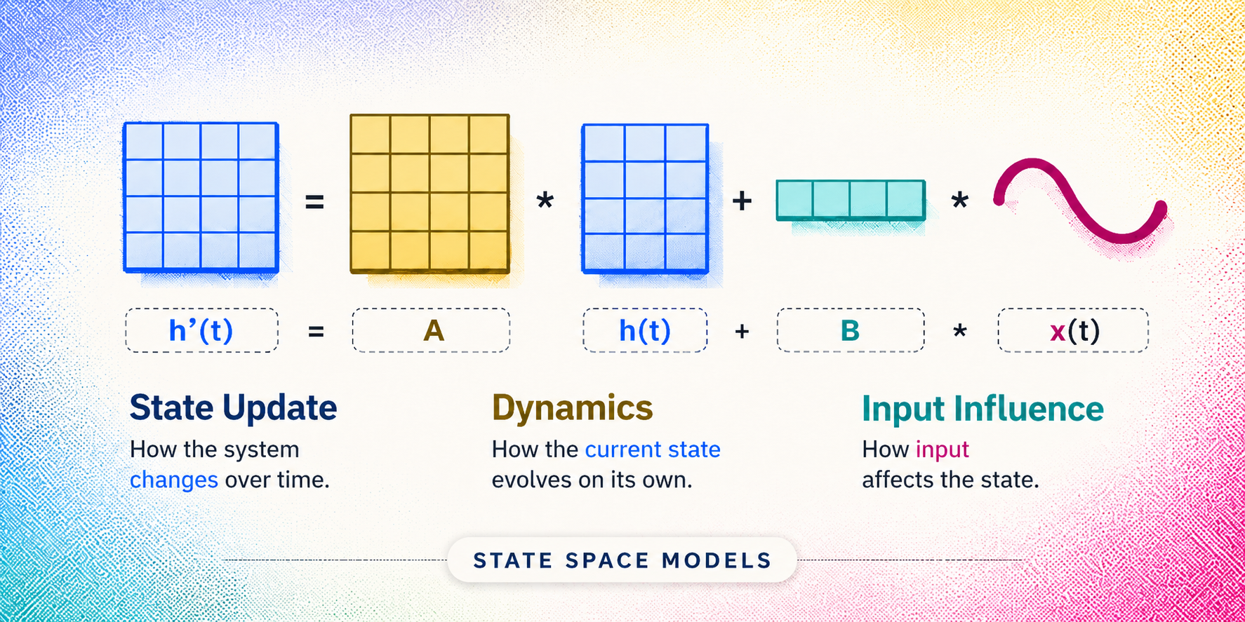
The SSM has three moving parts:
The two equations that define how the system evolves:
\(h'(t)\) is the derivative of the hidden state, the rate at which \(h\) is changing at time \(t\). It’s not a separate variable we store; it’s the velocity of the memory. The first equation says: the rate of change of the memory equals \(A\) times the current memory plus \(B\) times the current input. \(A\) is an \(N \times N\) matrix that controls how the state decays or mixes over time. \(B\) is an \(N \times 1\) matrix (a column vector) that decides how the input pushes into each dimension of the state. \(C\) is a \(1 \times N\) matrix (a row vector) that decides how to read out a scalar from the state.
A concrete example with \(N = 1\) (scalar state). Take \(A = -2\), \(B = 1\), \(C = 1\).
Scenario 1 (\(x = 0\), \(h = 5\)):
The \(A = -2\) term pulls \(h\) toward zero. With \(x = 0\), the derivative is just \(h' = -2 \cdot 5 = -10\), so the state is decreasing at rate 10 per unit time. Using the Euler approximation \(h(t + \delta) \approx h(t) + h'(t) \cdot \delta\) with \(\delta = 0.1\):
The derivative itself shrinks as \(h\) gets smaller, so the decay slows down over time but never quite reaches zero. That’s exponential decay. To find the exact formula, start from \(h' = -2h\) and rearrange:
Integrate both sides:
At \(t = 0\), \(h(0) = 5\), so \(e^C = 5\). Therefore \(h(t) = 5 \cdot e^{-2t}\):
| \(t\) | \(h(t) = 5 e^{-2t}\) |
|---|---|
| 0 | 5.00 |
| 0.25 | 3.03 |
| 0.5 | 1.84 |
| 1.0 | 0.68 |
| 2.0 | 0.09 |
The more negative \(A\) is, the faster it forgets.
Scenario 2 (\(x = 3\), \(h = 0\)):
The memory is rising. The input pushes new information into the state through \(B\). The state ramps up toward the equilibrium point, the value of \(h\) where the state stops changing (\(h' = 0\)). Setting \(h' = -2h + 3 = 0\) gives \(h = 1.5\). At that point, the decay (\(-2 \cdot 1.5 = -3\)) exactly cancels the input (\(+3\)), so \(h' = 0\). Recall the Euler update: \(h(t + \delta) = h(t) + h'(t) \cdot \delta\). When \(h' = 0\), this becomes \(h(t + \delta) = h(t) + 0 \cdot \delta = h(t)\). The state doesn’t move. Every subsequent step leaves it at 1.5, as long as \(x\) stays at 3.
Scenario 3, reading the output:
If \(h = 4.2\) and \(C = 1\), then \(y = 1 \cdot 4.2 = 4.2\). \(C\) is just a gain knob on the readout.
Scaling to multiple dimensions:
In the real model, \(h(t)\) is a vector of size \(N\), not a scalar. Each dimension has its own entry in \(A\) that controls its decay rate. \(A\) is always diagonal in Mamba: each state dimension decays independently, with no off-diagonal interaction. The recurrence implementation in code uses an elementwise multiply (A_bar * h), not a matrix multiply. The original S4 paper (Structured State Spaces for Sequence Modeling) allowed full structured \(A\) matrices which let state dimensions oscillate or mix, but Mamba simplifies to diagonal because the selectivity mechanism provides enough expressivity without it. Suppose we have \(N = 3\):
An input \(x = 5\) arrives. All three dimensions absorb it equally through \(B\). The input then stops (\(x = 0\)), and we watch the state decay:
Each dimension decays as \(h_i(t) = 5 \cdot e^{A_{ii} \cdot t}\) (same formula we derived earlier, with initial value 5 and no further input). For example, \(h_1\) at \(t = 0.5\): \(5 \cdot e^{-0.1 \cdot 0.5} = 5 \cdot e^{-0.05} = 5 \cdot 0.951 = 4.76\). And \(h_3\) at \(t = 0.5\): \(5 \cdot e^{-10 \cdot 0.5} = 5 \cdot e^{-5} = 5 \cdot 0.0067 = 0.03\).
| Time after input stops | \(h_1 = 5e^{-0.1t}\) (slow) | \(h_2 = 5e^{-1 \cdot t}\) (medium) | \(h_3 = 5e^{-10t}\) (fast) |
|---|---|---|---|
| \(t = 0\) | \(5 \cdot e^0 = 5.00\) | \(5 \cdot e^0 = 5.00\) | \(5 \cdot e^0 = 5.00\) |
| \(t = 0.5\) | \(5 \cdot e^{-0.05} = 4.76\) | \(5 \cdot e^{-0.5} = 3.03\) | \(5 \cdot e^{-5} = 0.03\) |
| \(t = 1.0\) | \(5 \cdot e^{-0.1} = 4.52\) | \(5 \cdot e^{-1} = 1.84\) | \(5 \cdot e^{-10} \approx 0\) |
| \(t = 3.0\) | \(5 \cdot e^{-0.3} = 3.70\) | \(5 \cdot e^{-3} = 0.25\) | \(\approx 0\) |
| \(t = 10.0\) | \(5 \cdot e^{-1} = 1.84\) | \(5 \cdot e^{-10} \approx 0\) | \(\approx 0\) |
\(h_3\) (the fast-decaying dimension) forgets the input almost immediately. It’s useful for very local patterns, like “the previous character was a vowel.” \(h_1\) (the slow-decaying dimension) still remembers 37% of the input after 10 time units. It’s useful for long-range patterns, like “we’re inside a paragraph that started with ROMEO.” \(h_2\) sits in between. The output \(y(t) = C h(t) = h_1 + h_2 + h_3\) blends all three timescales.
This is the key property of an SSM: a single recurrent layer with state size \(N\) can simultaneously track patterns at \(N\) different timescales, because each dimension of \(h\) acts like an independent exponentially-decaying memory with its own rate. Different timescales means different dimensions remember things from different points in the past: a slow dimension (\(A = -0.1\)) still holds traces of inputs from hundreds of steps ago, while a fast dimension (\(A = -10\)) only remembers the last few. Bigger \(N\) means more timescales the system can represent at once. In our model, \(N = 16\), so each channel has 16 parallel memories spanning short-range to long-range context.
Why not stay in continuous time?
An LLM processes tokens, which are discrete objects. Token 1, token 2, token 3. There is no “token 1.5” in between. The ODE \(h'(t) = Ah(t) + Bx(t)\) describes a system that flows smoothly through continuous time, but we don’t have a continuous signal to feed it. We have a sequence of discrete inputs.
To use this system for token sequences, we need to convert it into a step-by-step rule: “given the hidden state after token \(t-1\) and the new input \(x_t\), compute the hidden state after token \(t\).” That conversion is called discretization.
We have the continuous ODE \(h'(t) = Ah(t) + Bx(t)\), but we process tokens one at a time. We need a rule that says “given the state after token \(t-1\) and the new input \(x_t\), compute the state after token \(t\).” That rule comes from integrating the ODE forward by one step of size \(\Delta\).
Deriving \(\bar{A}\): Start with the ODE in the no-input case (\(x = 0\)): \(h' = Ah\). We already know how to solve this. Rearrange:
Integrate both sides:
At \(t = 0\), \(h(0) = e^C\), so \(h(t) = h(0) \cdot e^{At}\). After a time step of size \(\Delta\):
So the factor \(e^{A\Delta}\) is the fraction of the old state that survives after \(\Delta\) time. We call this \(\bar{A}\):
If \(A = -2\) and \(\Delta = 0.5\), then \(\bar{A} = e^{-1} = 0.37\). The state retains 37% per step. Starting from \(h = 1\):
| Step | \(h_t = 0.37 \cdot h_{t-1}\) |
|---|---|
| 0 | 1.0 |
| 1 | \(1.0 \times 0.37 = 0.37\) |
| 2 | \(0.37 \times 0.37 = 0.14\) |
| 3 | \(0.14 \times 0.37 = 0.05\) |
| 4 | \(0.05 \times 0.37 = 0.02\) |
The state smoothly decays toward zero. Every step keeps 37% of what was there before. Compare this to the Euler version below where the same \(A\) and \(\Delta\) values can produce explosion.
The Euler approximation would give \(h(t + \Delta) \approx h(t) + h'(t) \cdot \Delta\). Substituting \(h' = Ah\):
So Euler’s version of \(\bar{A}\) is \((1 + \Delta A)\), a linear approximation of the same survival fraction. For small \(\Delta\) the two agree: with \(A = -2\), \(\Delta = 0.1\), Euler gives \(1 + (0.1)(-2) = 0.8\) while the exact gives \(e^{-0.2} = 0.82\). Close enough.
But for larger \(\Delta\) it breaks catastrophically. Take \(A = -10\), \(\Delta = 0.5\), starting from \(h = 1\):
The exponential can never do this. Since \(A < 0\), \(e^{\Delta A}\) is always in \((0, 1)\): always positive, always less than 1, always a valid decay factor, no matter how large \(\Delta\) gets.
The diagonal structure: Since \(A\) is diagonal in Mamba (shape [D, N]), there’s no matrix exponential involved. Each state dimension decays independently:
In code this is just elementwise exp on the product of two tensors:
A_bar = torch.exp(delta_t.unsqueeze(-1) * A.unsqueeze(0)) # [B, D, N]Each entry A_bar[b, d, n] = \(e^{\Delta_{b,d} \cdot A_{d,n}}\) is the survival fraction for that specific (batch, channel, state-dim). Dimension 1 might retain 90% while dimension 16 retains 0.1%. No cross-dimension interaction, no matrix math.
The full discretized recurrence: Adding back the input term (under the “zero-order hold” assumption that \(x\) is constant over the interval \(\Delta\)), the discrete update becomes:
The output is still \(y_t = C h_t\). No more calculus, no more derivatives. Multiply the old state by \(\bar{A}\), add \(\bar{B}\) times the new input, done.
A scalar example: Take \(A = -2\), \(B = 1\), \(\Delta = 0.5\).
So the update rule becomes: \(h_t = 0.37 \cdot h_{t-1} + 0.5 \cdot x_t\). Keep 37% of the old state, add half the new input. Run it starting from \(h_0 = 0\), with input \(x_1 = 5\) at step 1 and nothing afterward:
| Step | \(x_t\) | \(h_t = 0.37 \cdot h_{t-1} + 0.5 \cdot x_t\) | What happened |
|---|---|---|---|
| 1 | 5 | \(0.37 \cdot 0 + 0.5 \cdot 5 = 2.5\) | Input absorbed |
| 2 | 0 | \(0.37 \cdot 2.5 + 0.5 \cdot 0 = 0.92\) | Decaying |
| 3 | 0 | \(0.37 \cdot 0.92 = 0.34\) | Still decaying |
| 4 | 0 | \(0.37 \cdot 0.34 = 0.13\) | Almost forgotten |
The state absorbed the input then exponentially decayed. \(\bar{A} = 0.37\) is the per-step retention rate.
The big idea, \(\Delta\) is a knob: So far we’ve kept \(\Delta\) constant. But what if we vary it? Same \(A = -2\) and \(B = 1\), single input \(x = 5\) from a zero starting state, but now try different \(\Delta\) values:
| \(\Delta\) | \(\bar{A} = \exp(\Delta A)\) | \(\bar{B} = \Delta B\) | \(h_1 = \bar{A} \cdot 0 + \bar{B} \cdot 5\) | Interpretation |
|---|---|---|---|---|
| 0.01 (tiny) | \(\exp(-0.02) = 0.98\) | 0.01 | 0.05 | Almost ignored the input. State barely moved. |
| 0.5 (medium) | \(\exp(-1.0) = 0.37\) | 0.5 | 2.5 | Absorbed a moderate amount. |
| 5.0 (huge) | \(\exp(-10) \approx 0\) | 5.0 | 25.0 | Wiped the old state, slammed the input in. |
Small \(\Delta\): the model is saying “this token doesn’t matter, keep what I have.” \(\bar{A} \approx 1\) (retain everything from past), \(\bar{B} \approx 0\) (absorb nothing).
Large \(\Delta\): the model is saying “this token is important, reset and absorb it.” \(\bar{A} \approx 0\) (forget everything from past), \(\bar{B}\) is large (absorb strongly).
\(\Delta\) interpolates smoothly between “ignore this token” and “let this token completely overwrite the state.” This is exactly why \(\Delta\) becomes the central lever for selectivity when Mamba makes it input-dependent in the next section.
In code, the discretization happens inside the per-token loop, computed fresh for every token:
A_bar = torch.exp(delta_t.unsqueeze(-1) * A.unsqueeze(0))   # [B, D, N]
B_bar = delta_t.unsqueeze(-1) * B_t.unsqueeze(1)            # [B, D, N]
h = A_bar * h + B_bar * x_t.unsqueeze(-1)                   # [B, D, N]
The first two lines are \(\bar{A} = \exp(\Delta A)\) and \(\bar{B} = \Delta B\). The third is the recurrence \(h_t = \bar{A} h_{t-1} + \bar{B} x_t\). All multiplies are elementwise.
Why We Store A_log Instead of A ?In the code, you’ll notice we never store \(A\) directly as a parameter. Instead we store a tensor called A_log and compute \(A = -\exp(\texttt{A\_log})\) on the fly. Why?
We don’t make the optimizer respect it. We let the optimizer push any number it wants into a raw parameter, and apply a function on top that guarantees the result is always a valid \(A\).
In the code:
a = torch.log(torch.arange(1, d_state + 1, dtype=torch.float32))  # [N]
self.A_log = nn.Parameter(a.unsqueeze(0).repeat(d_inner, 1).contiguous())  # [D, N]
and later, every forward pass starts with:
A = -torch.exp(self.A_log.float()) # [D, N], negative real eigenvaluesA_log is a learnable tensor of shape [d_inner, d_state], one entry per (channel, state-dimension) pair. The actual \(A\) used in the recurrence is \(-\exp(\texttt{A\_log})\), which is always negative no matter what numbers A_log contains. We need \(A\) to be negative because it controls how much the state forgets per step: \(\bar{A} = e^{\Delta A}\), and only negative \(A\) gives \(\bar{A} \in (0, 1)\) (a valid decay factor). A positive \(A\) would give \(\bar{A} > 1\), meaning the state grows every step and eventually explodes. The optimizer is free to roam the entire real line; the \(-\exp(\cdot)\) guarantees we never accidentally end up there.
There’s a second reason this parameterization helps. Consider two channels: one with \(A = -1\) (slow decay, remembers far back) and one with \(A = -100\) (fast decay, only sees the last token or two). If we stored \(A\) directly and the optimizer applied the same step of \(-0.5\) to both:
The same gradient step has wildly different effects depending on the magnitude of \(A\). The optimizer can’t find a single learning rate that works for both.
By storing \(\log|A|\) instead, an additive step in log-space becomes a multiplicative step in real space. Say the optimizer adds \(+0.1\) to A_log:
A_log starts at \(\ln(1) = 0\). Optimizer adds \(0.1\): A_log becomes \(0 + 0.1 = 0.1\). So \(A = -e^{0.1} = -1.105\). Changed from \(-1\) to \(-1.105\), a 10.5% increase.A_log starts at \(\ln(100) = 4.605\). Optimizer adds \(0.1\): A_log becomes \(4.605 + 0.1 = 4.705\). So \(A = -e^{4.705} = -110.5\). Changed from \(-100\) to \(-110.5\), a 10.5% increase.Both channels get adjusted by the same proportion, so the optimizer sees uniformly-behaved gradients regardless of the magnitude of \(A\).
The initialization is on purpose: The arange(1, d_state+1) part is what gives us 16 channels with eigenvalues \(-1, -2, \ldots, -16\) at the start of training:
A = -exp(log([1, 2, 3, ..., 16]))
  = -[1, 2, 3, ..., 16]
After discretization, the per-step retention rate for state dimension \(k\) is \(\bar{A}_k = \exp(\Delta \cdot A_k) = \exp(\Delta \cdot (-k))\). This is the fraction of that dimension’s state that survives one step. With \(\Delta = 1\):
| State dim \(k\) | \(A_k\) | \(\bar{A}_k = \exp(1 \cdot A_k)\) | Meaning |
|---|---|---|---|
| 1 | -1 | \(e^{-1} = 0.368\) | Retains 36.8% per step. After 2 steps: \(0.368^2 = 0.135\). After 5 steps: \(0.368^5 = 0.007\). Slow forgetting. |
| 2 | -2 | \(e^{-2} = 0.135\) | Retains 13.5% per step. After 2 steps: \(0.135^2 = 0.018\). Forgets most things within 2-3 steps. |
| 4 | -4 | \(e^{-4} = 0.018\) | Retains 1.8% per step. Essentially gone after a single step. |
| 8 | -8 | \(e^{-8} = 3.4 \times 10^{-4}\) | Retains 0.03% per step. Only reacts to the current token. |
| 16 | -16 | \(e^{-16} = 1.1 \times 10^{-7}\) | Retains essentially nothing. The state is almost entirely determined by the current input. |
Dimension 1 is the “long memory” dimension: it holds onto 37% of the previous state each step, so information from 5-10 steps ago still has a trace. Dimension 16 is the “instant” dimension: it forgets everything from the previous step and only reflects the current token through \(\bar{B} \cdot x_t\). Together, the 16 dimensions give the model access to information at 16 different time horizons simultaneously.
We start training with a spread of timescales already baked in. State dim 1 holds onto things for many steps, state dim 16 forgets almost instantly. The optimizer can then adjust these rates during training, but it doesn’t have to discover from scratch that the model needs both fast and slow dimensions.
The A_log tensor has shape [256, 16]: 256 dimensions of d_inner (the expanded representation inside each block), each with 16 state dimensions. At initialization, every one of the 256 gets the same 16 decay rates [-1, -2, ..., -16]. Dimension 0 has the same A values as dimension 1, dimension 2, etc. They all start identical.
How do they become different during training? Through in_proj. It’s a [512, 128] weight matrix (we only care about the first 256 rows here, the SSM path). When a token’s 128-dim embedding arrives, the matrix multiply produces x_in, the 256-dim vector that will flow through conv and then into the SSM as input:
Each \(x\_in_d\) is a dot product of row \(d\) with the token’s embedding: \(x\_in_d = W_{d,0} \cdot \text{emb}_0 + W_{d,1} \cdot \text{emb}_1 + \ldots + W_{d,127} \cdot \text{emb}_{127}\).
After passing through the conv and SiLU, this value becomes the \(x_t[d]\) that the SSM absorbs into its hidden state at dimension \(d\):
The full hidden state has shape [256, 16]: 256 dimensions, each with 16 state slots. At every time step, all 256 dimensions update in parallel:
But each \(h_t[d]\) above is not a scalar, it’s a vector of 16 slots. Here’s what happens inside each index \(d\):
The update for all 16 slots in dimension \(d\):
For a single slot \(n\) within dimension \(d\), written out:
Where each part comes from:
- \(\bar{A}[d, n] = e^{\Delta_t[d] \cdot A[d, n]}\): the decay factor. \(A[d,n]\) is a learned negative number (from A_log), \(\Delta_t[d]\) is the step size the current token chose. Together they produce a number between 0 and 1 that controls forgetting.
- \(h_{t-1}[d, n]\): whatever this slot accumulated from all previous tokens.
- \(\bar{B}[d, n] = \Delta_t[d] \cdot B_t[n]\): the input gate. \(B_t[n]\) is produced by x_proj from the current token, scaled by \(\Delta_t[d]\).
- \(x_t[d]\): the signal in_proj created for dimension \(d\) (after conv and SiLU).
A concrete example for dimension \(d = 3\). We’ll compare slot 0 (slowest decay) and slot 15 (fastest decay) to show the effect of different \(\bar{A}\) values. Assume both started with \(h_{t-1} = 2.0\), and the current input is \(x_t[3] = 1.5\):
| Slot 0 (slow) | Slot 15 (fast) | |
|---|---|---|
| decay rate \(\bar{A} = e^{\Delta \cdot A}\) | \(e^{0.5 \times (-1)} = 0.61\) | \(e^{0.5 \times (-16)} = 0.0003\) |
| old state \(\times\) decay | \(0.61 \times 2.0 = 1.22\) | \(0.0003 \times 2.0 = 0.0006\) |
| new input \(\times\) \(\bar{B}\) | \(0.4 \times 1.5 = 0.6\) | \(0.4 \times 1.5 = 0.6\) |
| new state | 1.82 | 0.6006 |
Slot 0 kept most of its old state (1.22 out of 2.0) plus the new input. Slot 15 wiped its old state (0.0006 out of 2.0) and only has the fresh input. Same input, same dimension, different timescales.
The output for dimension \(d\) then reads from all 16 slots:
\(C_t\) (produced from the current token by x_proj) decides how to blend the 16 timescales into a single output value. This happens independently for all 256 dimensions, giving a 256-dim output vector \(y_t\).
So different rows of in_proj → different values of \(x_t[d]\) → different information gets written into different SSM dimensions. Row 0 has its own 128 weights, row 50 has different 128 weights, so they pick up different things from the same token and feed different signals into their respective SSM dimensions.
At initialization the weights are random (small gaussian, std=0.02), so each of the 256 dimensions starts by picking up an arbitrary mix of the 128 input features. During training, backprop tunes each row independently, so each dimension gradually specializes: one might become sensitive to punctuation, another to uppercase letters, another to spacing patterns. Over time, the optimizer also adjusts each dimension’s A_log entries independently. Dimension 0 might end up with faster decay rates than it started with, while dimension 50 might slow down. But the key point of the [1, 2, ..., 16] initialization is that every dimension already has a useful spread of decay rates from step 0: some state slots that forget quickly, some that remember for a long time. Without this, the model would start with all decay rates at the same value and would have to spend early training steps just figuring out that it needs different timescales, before it can even start learning patterns in the data.
In the original S4 paper, \(A\), \(B\), \(C\), and \(\Delta\) were all fixed model parameters. The same dynamics applied to every token regardless of content. That gave the model nice mathematical properties (as we saw earlier, a fixed recurrence reduces to a convolution that you can compute in parallel) but limited quality, because the model couldn’t react to its input.
Mamba changes this by making \(B\), \(C\), and \(\Delta\) functions of the current input \(x_t\). \(A\) stays fixed across tokens (this preserves the \(-\exp(\cdot)\) parameterization above), but the other three flow from a linear projection of the input:
self.x_proj = nn.Linear(d_inner, self.dt_rank + 2 * d_state, bias=False)  # [256] -> [16 + 2*16 = 48]
self.dt_proj = nn.Linear(self.dt_rank, d_inner, bias=True)                # [16] -> [256]
x_proj takes the input vector of size d_inner and produces a tensor of size dt_rank + 2 * d_state, which gets split three ways. The first dt_rank entries are a low-rank version of \(\Delta\), and the next two d_state-sized chunks are \(B\) and \(C\):
x_dbl = self.x_proj(x)                            # [B, L, 48]
delta_low, B_proj, C_proj = torch.split(
    x_dbl, [self.dt_rank, N, N], dim=-1            # [B, L, 16], [B, L, 16], [B, L, 16]
)
Then dt_proj lifts \(\Delta\) from dt_rank back up to d_inner, giving every channel its own per-token timescale:
delta = F.softplus(self.dt_proj(delta_low)).float() # [B, L, 256], positiveA few things to notice here.
The low-rank trick for \(\Delta\): If we projected \(x\) directly to a \(\Delta\) of size d_inner, we’d need a weight matrix of shape [d_inner, d_inner], which is 256 * 256 = 65,536 parameters per MambaBlock (and we have 6 blocks, so that adds up). Instead, we project down to dt_rank = max(d_inner // 16, 1) = 16 first and then lift back up. That’s d_inner * dt_rank + dt_rank * d_inner = (256 * 16) * 2 = 8,192 parameters per block, an 8x reduction with no real loss of expressivity (in practice, the per-token \(\Delta\) doesn’t need a full 256-dimensional description of the input to be computed well; 16 numbers summarize it just fine).
Softplus keeps \(\Delta\) positive: The linear projections (x_proj → dt_proj) already make \(\Delta\) input-dependent, which is the whole point of selectivity: each token gets to choose its own step size. But those linear layers can output any real number, and \(\Delta\) must be positive (it’s a step size; negative makes no sense). Softplus, defined as \(\text{softplus}(x) = \log(1 + e^x)\), smoothly maps the entire real line to positive numbers without a hard cutoff like ReLU. It’s purely a constraint on the output, not the mechanism that creates input-dependence.
\(B\) and \(C\) have no further activation: They come directly out of x_proj as unconstrained real numbers. \(B\) is the “input gate” deciding which dimensions of the state absorb the input, and \(C\) is the “output gate” deciding which dimensions are read out. Both can be positive or negative, so no activation is needed.
Why no bias on x_proj but yes on dt_proj? \(B\) and \(C\) are meant to be functions of the input that go to zero when the input is zero (an empty input shouldn’t gate anything in or out). \(\Delta\), in contrast, needs a sensible default value even for “boring” inputs; the bias provides that resting timescale.
To see why selectivity matters, contrast it with a fixed recurrence. Imagine \(\Delta\) is hard-coded to \(0.5\) for every token. Now feed in "the quick brown fox jumps over the lazy dog". The model has no way to say “the word the is filler, don’t bother updating the state much” vs “the word fox is a content word, reset and absorb it.” Every token gets the same update with \(\bar{A} = 0.37\) and \(\bar{B} = 0.5\).
What does that look like concretely? The full \(h_t\) (hidden state) per token is a [256, 16] matrix, but suppose we track just one slot in one dimension:
| Token | \(h\) before | decay (\(\times 0.37\)) | new input (\(\times 0.5\)) | \(h\) after |
|---|---|---|---|---|
| “the” | 0 | 0 | \(0.5 \times 2.1 = 1.05\) | 1.05 |
| “quick” | 1.05 | 0.39 | \(0.5 \times 3.0 = 1.50\) | 1.89 |
| “brown” | 1.89 | 0.70 | \(0.5 \times 2.8 = 1.40\) | 2.10 |
| “fox” | 2.10 | 0.78 | \(0.5 \times 4.2 = 2.10\) | 2.88 |
Every token gets blended in with the same weight (0.5) and the past decays at the same rate (0.37), regardless of whether the token is important or not. The state is just a smoothed running average where recent tokens dominate and old ones fade exponentially. The model can’t “pay attention” to fox more than the.
With input-dependent \(\Delta\), the model can produce a small \(\Delta\) for the (state nearly unchanged) and a large \(\Delta\) for fox (state reset, new info absorbed). Selectivity is exactly the analog of attention’s “decide where to look”, but expressed inside a recurrent update rather than a softmax over keys.
The price you pay for selectivity is real but understandable. With \(B\), \(C\), \(\Delta\) all input-dependent, the recurrence is no longer linear time-invariant. You can’t precompute it as a single global convolution (as we saw earlier). You have to actually run the recurrence step by step. The Mamba paper introduces a hardware-aware parallel scan that runs this in \(O(L)\) work but with parallelism across \(L\) on the GPU. For our minimal implementation we stick with the sequential Python loop. It’s slower but the structure is much easier to read.
Causality, for free: The recurrence has a nice structural property: nothing in the loop ever looks at future inputs. At step \(t\), the computation reads only delta[:, t], B[:, t], C[:, t], and x[:, t]. Past information flows in through h (produced by previous steps). Future information has no path to the current output. This is causality by construction; there’s no triangular mask like in attention.
The selective SSM is the core, but a Mamba block wraps several things around it that make a big practical difference. Here’s the full block:
class MambaBlock(nn.Module):
    def __init__(self, d_model, d_state=16, d_conv=4, expand=2):
        super().__init__()
        d_inner = expand * d_model
        self.d_inner = d_inner
        self.d_conv = d_conv
        self.norm = RMSNorm(d_model)
        self.in_proj = nn.Linear(d_model, 2 * d_inner, bias=False)
        self.conv = nn.Conv1d(
            in_channels=d_inner,
            out_channels=d_inner,
            kernel_size=d_conv,
            groups=d_inner,
            padding=d_conv - 1,
        )
        self.ssm = SelectiveSSM(d_inner=d_inner, d_state=d_state)
        self.out_proj = nn.Linear(d_inner, d_model, bias=False)

    def forward(self, x: torch.Tensor) -> torch.Tensor:
        # x: [B, L, d_model] = [64, 256, 128]
        residual = x
        x = self.norm(x)                                 # [B, L, d_model] = [64, 256, 128]

        xz = self.in_proj(x)                             # [B, L, 2*D] = [64, 256, 512]
        x_in, z = xz.chunk(2, dim=-1)                    # each: [B, L, D] = [64, 256, 256]

        L = x_in.shape[1]
        x_c = x_in.transpose(1, 2)                       # [B, D, L] = [64, 256, 256]
        x_c = self.conv(x_c)[..., :L]                    # [64, 256, 256] (causal crop)
        x_c = x_c.transpose(1, 2)                        # [B, L, D] = [64, 256, 256]
        x_c = F.silu(x_c)

        y = self.ssm(x_c)                                # [B, L, D] = [64, 256, 256]
        y = y * F.silu(z)                                # [64, 256, 256] (multiplicative gate)
        out = self.out_proj(y)                           # [B, L, d_model] = [64, 256, 128]

        return residual + out
We already saw that in_proj projects each token from d_model = 128 into a 256-dim vector that flows through conv and SiLU into the SSM. But looking at the full block, in_proj actually outputs 2 * d_inner = 512 dimensions, which get chunked into two halves: x_in (the SSM path we traced earlier) and z (a gated branch we haven’t seen yet).
The block starts with RMSNorm (a cheaper LayerNorm that skips mean subtraction, standard in modern transformers) for training stability. Then x_in passes through a depthwise causal convolution before the SSM:
self.conv = nn.Conv1d(
    in_channels=d_inner, out_channels=d_inner,
    kernel_size=d_conv, groups=d_inner, padding=d_conv - 1,
)
Why a convolution before the SSM? The SSM sees past tokens through its hidden state, but that view is controlled by the gated recurrence (the information has been compressed, decayed, and mixed across state dimensions). The conv gives the model a direct shortcut to local context. In practice, having both paths helps quality significantly.
What “depthwise” means: A regular convolution mixes all input channels together: each output channel is a weighted sum over all input channels at each position. A depthwise convolution (groups=d_inner) keeps channels independent: each of the 256 channels has its own tiny filter, and no cross-channel mixing happens. That’s a 256x parameter reduction (256 filters of size 4 = 1,024 parameters, vs 256×256×4 = 262,144 for a regular conv). Cross-channel mixing is handled by in_proj and out_proj, the linear layers before and after.
Why the transposes? Look at the code: we call .transpose(1, 2) before the conv and again after. This is because nn.Conv1d wants each row to be a channel and each column to be a time step (it slides its kernel along columns). But the rest of our network stores data the other way: each row is a token and each column is a channel. A quick example with 4 tokens and 3 channels:
Our layout [B, L, D]:            Conv1d's layout [B, D, L]:

        ch0  ch1  ch2                    t0   t1   t2   t3
 t0  [  1.0  2.0  3.0 ]          ch0  [  1.0  0.5  2.0  1.0 ]
 t1  [  0.5  1.5  0.0 ]          ch1  [  2.0  1.5  3.0  0.5 ]
 t2  [  2.0  3.0  1.0 ]          ch2  [  3.0  0.0  1.0  2.0 ]
 t3  [  1.0  0.5  2.0 ]
Same numbers, just rows and columns swapped. The first transpose gives the conv what it expects, and the second transpose puts things back for the rest of the block.
A concrete example. Suppose d_inner = 3 (three channels) and kernel_size = 4. Each channel has its own 4-element filter. Consider two channels of a 6-token input:
Channel 0 input:  [2.0, 1.0, 3.0, 0.5, 2.0, 1.5]
Channel 0 filter: [0.1, 0.3, 0.2, 0.4]

Channel 1 input:  [1.0, 0.0, 2.0, 1.0, 0.5, 3.0]
Channel 1 filter: [0.5, 0.1, 0.2, 0.2]
Each filter slides along its own channel only. At position \(t = 3\) (the fourth token), channel 0 computes:
Channel 1 at the same position computes a completely different weighted sum of its own values:
Channel 0’s output depends only on channel 0’s input. Channel 1 never sees channel 0’s values. Each channel independently blends its last 4 tokens with its own learned weights. One channel might learn to detect “was there a capital letter in the last 4 positions?” while another detects “was there a space recently?”
What “causal” means: For a language model, position \(t\)’s output must not depend on future tokens. The conv achieves this through padding and cropping:
Input positions:      [0,  1,  2,  3,  4,  5]
Padded (3 zeros):  [0, 0, 0,  0,  1,  2,  3,  4,  5,  0,  0,  0]
                    ← left pad →                      ← right pad →
After the kernel-4 convolution slides across, the output has length \(L + 3 = 9\). The [..., :L] crop keeps only the first 6 positions, discarding the rightward padding’s contribution. The result: position \(t\) depends on inputs \([t-3, t-2, t-1, t]\), only past and present. No future leaks in.
Without the crop, position 6 would see padded zeros from the right, which don’t cause information leakage (zeros carry no information) but do produce extra output positions we don’t need. The left padding ensures even position 0 has a well-defined output: its kernel window is [0, 0, 0, input[0]], three zero-pads and the current token.
After the SSM, the output is multiplied elementwise by SiLU(z):
y = self.ssm(x_c)                                # [B, L, D]
y = y * F.silu(z)                                # multiplicative gate
Remember that in_proj produced two halves: x_in went through the conv and SSM, while z skipped all of that. Now z acts as a gate: SiLU(z) produces a value between roughly 0 and 1 for each (token, channel) pair. Multiplying by it lets the model turn individual channels on or off per token. If the SSM output for some channel isn’t useful at a particular position, the gate can suppress it to near zero without the SSM itself having to learn to output zero. This gating pattern (called GLU) is also used in transformer FFNs (SwiGLU in Llama, GeGLU in PaLM).
Note the two different dimensions here. “Channel” refers to the 256 d_inner features: in_proj expands each token from 128 to 256 dimensions, and each of those 256 channels runs its own independent SSM. The gate operates at this level, choosing which channels to keep or suppress. Inside each channel’s SSM there is a separate d_state = 16 hidden state, the 16 memory slots that let that channel track information across different time-scales. So 256 channels times 16 slots = 4,096 total state values per token.
Finally, out_proj compresses back from d_inner = 256 to d_model = 128 and the result is added to the residual from the top of the block. This residual connection is what makes blocks stackable: each contributes a delta, and stacking more blocks accumulates more refinements.
The full model is an embedding, a stack of Mamba blocks, a final norm, and an LM head:
x = self.embedding(idx)                          # [B, L, d_model] = [64, 256, 128]
for blk in self.blocks:                          # 4 MambaBlocks
    x = blk(x)
x = self.norm_f(x)                               # [B, L, d_model] = [64, 256, 128]
logits = self.lm_head(x)                         # [B, L, vocab]   = [64, 256, 65]
The structure follows a common pattern in language models. The embedding turns each token id into a dense vector the network can work with. The Mamba blocks (described in the previous sections) are where all the learning happens: each block refines the representation by mixing in information from past tokens (via the SSM and conv), and stacking 4 of them lets the model build increasingly abstract features, the same reason deep networks outperform shallow ones. The final norm stabilizes the representations, and the LM head converts each 128-dim vector into 65 scores (one per character in our vocabulary). The embedding and LM head share the same weight matrix (weight tying): both are [65, 128], one mapping token ids to vectors, the other mapping vectors back to scores (logits).
The loss function: The LM head produces 65 raw scores per position, called logits. To train the model we need to measure how wrong these scores are, and that’s what cross-entropy loss does:
loss = F.cross_entropy(
    logits.view(-1, vocab_size),                 # [B*L, vocab] = [16384, 65]
    targets.view(-1),                            # [B*L]        = [16384]
)
For each of the 16,384 positions (64 sequences in the batch, each 256 tokens long), the loss computes \(-\log(p_{\text{correct}})\): softmax converts the 65 logits into probabilities, and then we only look at the probability assigned to the correct next character. If the model puts 90% on the right character, \(-\log(0.9) = 0.105\), a small loss. If it spreads probability evenly across all 65 characters, \(-\log(1/65) = \ln(65) \approx 4.17\), which is also where an untrained model starts. The final loss is the average across all 16,384 positions, giving a single scalar that gradients flow back through.
After training, we sample 500 characters from the prompt ROMEO::
@torch.no_grad()
def generate(self, idx, max_new_tokens, temperature=1.0):
    for _ in range(max_new_tokens):
        logits, _ = self(idx)
        logits = logits[:, -1, :].float() / max(temperature, 1e-8)
        probs = F.softmax(logits, dim=-1)
        next_id = torch.multinomial(probs, num_samples=1)
        idx = torch.cat([idx, next_id], dim=1)
    return idx
The flow is straightforward:
logits[:, -1, :]), which represent the model’s prediction for the next character.temperature (lower = more deterministic, higher = more random).torch.multinomial.Why sample instead of picking the best? We could use torch.argmax to always pick the highest-probability character (greedy decoding), but that produces repetitive, boring text because the model gets stuck in high-probability loops. Sampling from the distribution gives variety: a character with 30% probability gets picked roughly 30% of the time.
After 50000 steps of training, here’s how generation works character by character from the prompt ROMEO::
Input: "ROMEO:" - model predicts next char → samples "\n"
Input: "ROMEO:\n" - model predicts next char → samples "W"
Input: "ROMEO:\nW" - model predicts next char → samples "h"
Input: "ROMEO:\nWh" - model predicts next char → samples "a"
...500 steps later, all sampled characters appended together:
ROMEO:
What is thou speak: Romeo, sir? thank you
Did I make you that to me my fair daughter,
That love'd a may by some pace.
JULIET:
Marry, must you, sir, here is a most by
The hour of seven, this is the hand of...The model isn’t writing real Shakespeare; it has no idea what a plot is, and the syntax breaks down on close inspection. But it’s learned the surface form: character names with colons, line breaks at appropriate places, archaic vocabulary, blank-verse-ish cadence. For a 0.5M-parameter model trained for 25 minutes on a single GPU, that’s pretty impressive.
This post covers the intuition behind state space models and Mamba: why compressing the past into a fixed-size hidden state is a useful alternative to attention, what the continuous-time ODE looks like, how discretization turns it into a recurrence you can run on tokens, and why making the parameters input-dependent (selectivity) is the key idea that makes Mamba work where earlier SSMs fell short. Every concept is explained with actual PyTorch code snippets so you can see not just the math but how each equation maps to actual tensors and operations.
This is an educational implementation, not a production one. It skips the fused CUDA kernel that makes real Mamba fast (our Python loop does the same math, just 5-20x slower), doesn’t cache hidden states between generation steps, doesn’t cover Mamba-2 (which restructures the SSM as structured masked attention), and runs at toy scale (491K parameters, 65-character vocab) rather than the billions of parameters and subword tokenizers used in practice.
