Gaussian Splatting From Scratch: Explained Through Code

Karthik Ragunath Ananda Kumar

I built a minimal Gaussian Splatting implementation in pure PyTorch to understand how it actually works. This post goes through that code and explains what each piece does, why it's there, and how it all fits together.

The Big Picture

3D Gaussian Splatting represents a 3D scene as a collection of small, colored, semi-transparent blobs (3D Gaussians). To render an image from any viewpoint, you project those blobs onto the camera's image plane and blend them together front-to-back. Because every operation in this pipeline is differentiable, you can compare the rendered image to a real photograph and backpropagate the error to adjust every Gaussian's position, shape, color, and opacity.

The training loop is simple:

1. Start with a sparse point cloud from COLMAP (a Structure-from-Motion tool that recovers camera poses and 3D points from a set of photos).
2. Place one Gaussian at each point.
3. Repeat thousands of times: pick a training photo, render the scene from that camera, compute the difference from the real photo, backpropagate, update parameters.
4. Periodically add new Gaussians where the reconstruction is poor, and remove ones that have become transparent.

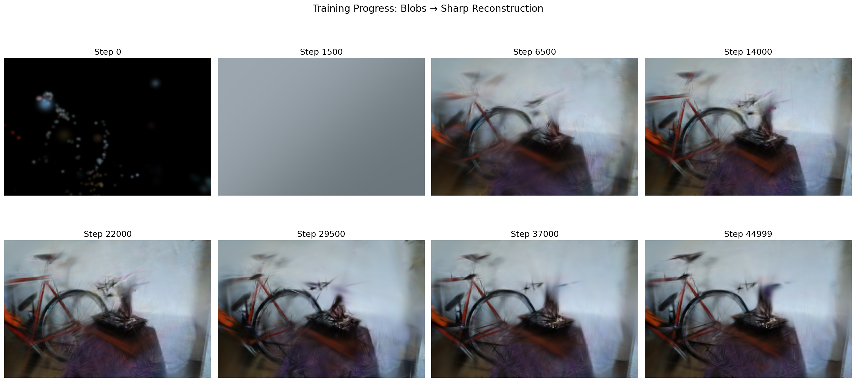
Here's what that looks like in practice. At step 0, the Gaussians are just scattered points from the initial point cloud. By step 1500 (right after the first opacity reset), the image is a gray wash because every Gaussian was just slammed to near-transparent. Over the next several thousand steps, structure emerges: rough shapes by step 6500, recognizable objects by step 14000, and progressively sharper detail through to step 44999.

After training, you have a collection of Gaussians that can be rendered from any viewpoint.

What Is a 3D Gaussian?

Each Gaussian in the scene is defined by five learnable properties. Here's how GaussianModel stores them:

class GaussianModel(nn.Module):
    def __init__(self):
        super().__init__()
        self._xyz = None             # [N, 3] position (mean) in world space
        self._log_scales = None      # [N, 3] log of scale along each axis
        self._rotations = None       # [N, 4] rotation as a quaternion (w, x, y, z)
        self._colors_raw = None      # [N, 3] raw color (before sigmoid)
        self._opacities_raw = None   # [N]    raw opacity (before sigmoid)

The values stored internally (the _xyz, _log_scales, etc. fields) are not the final values that get used during rendering. They are "raw" numbers that the optimizer is free to set to anything. When the rest of the code needs the actual scale, color, or opacity, it calls a property that converts the raw number into a valid one. Think of it as a two-step process: the model stores a "behind-the-scenes" number, and a mathematical function turns it into the "real" value on demand:

@property
def scales(self):
    return torch.exp(self._log_scales)       # always positive
 
@property
def rotations(self):
    return F.normalize(self._rotations, dim=-1)  # unit quaternion
 
@property
def colors(self):
    return torch.sigmoid(self._colors_raw)   # in [0, 1]
 
@property
def opacities(self):
    return torch.sigmoid(self._opacities_raw)  # in [0, 1]

Why the indirection? Consider scale. A Gaussian's scale must always be positive (you can't have a blob with negative size). Why not just store scales directly and let the optimizer update it? Because the optimizer does param = param - lr * gradient. If the current scale is 0.02 and the gradient update subtracts 0.05, you get -0.03, a negative scale, which is physically meaningless. You'd have to manually clamp it back to some small positive number after every step, which distorts the gradient signal and creates a hard wall the optimizer keeps crashing into.

There's a second problem: scale spans a huge range. Imagine two Gaussians: a tiny one with scale 0.001 (a sharp detail like a leaf edge) and a big one with scale 5.0 (a broad patch of wall). Now the optimizer applies the same step size of 0.01 to both:

If we store scale directly:

• Big Gaussian: 5.0 → 4.99. Changed by 0.2%. Barely moved. Fine.
• Tiny Gaussian: 0.001 → -0.009. Changed by 1000%. Went negative. Broken.

The same step is negligible for the big one and catastrophic for the small one. There's no single learning rate that works for both.

If we store log(scale) instead:

• Big Gaussian: log_scale = 1.609 → 1.609 - 0.01 = 1.599 → exp(1.599) = 4.95. Shrank by ~1%.
• Tiny Gaussian: log_scale = -6.908 → -6.908 - 0.01 = -6.918 → exp(-6.918) = 0.000990. Shrank by ~1%.

The same step of 0.01 in log-space shrinks both Gaussians by roughly the same percentage. In log-space, additive updates become multiplicative in real space. A step of -0.1 always means "shrink by ~10%", whether the Gaussian is huge or microscopic.

So we store _log_scales (which can be any real number: -10, 0, 5, anything) and recover the actual scale with exp(). For example:

No matter what value the optimizer assigns to _log_scales, exp() always produces a valid positive number. The optimizer is free to roam the entire real number line without ever producing an illegal scale.

Same idea for colors and opacity via sigmoid(). Opacity must be between 0 and 1. If we stored it directly, the optimizer could push it to 1.3 or -0.5 (both meaningless). Instead, we store _opacities_raw (unconstrained) and apply sigmoid:

The optimizer can push _opacities_raw to any value whatsoever, and sigmoid() guarantees the result is always a valid opacity in (0, 1). This "store unconstrained, activate with a function" pattern is standard in deep learning. It lets gradient descent work without constraints while the activation function enforces the physical requirements.

So far we have position, scale, rotation, color, and opacity. But to actually render a Gaussian, we need to know its full 3D shape, and that shape is described by a covariance matrix.

Why a covariance matrix? Think about what a single 3D Gaussian looks like. If it has equal scale in all directions and no rotation, it's a sphere. But most Gaussians in a scene aren't spheres. A Gaussian representing a piece of a wall might be flat (big in X and Y, thin in Z). One on a tree branch might be elongated (big in one direction, small in the other two). To describe these stretched, rotated ellipsoid shapes, we need something more than just "three scale numbers."

The covariance matrix $\Sigma$ is a 3x3 matrix that encodes all of this: how much the Gaussian spreads along each direction, and how those directions are oriented. It fully describes the ellipsoid's shape and orientation.

• A sphere has a covariance like $\begin{bmatrix} 1 & 0 & 0 \\ 0 & 1 & 0 \\ 0 & 0 & 1 \end{bmatrix}$: equal spread, no tilt.
• A pancake (flat disc) might have $\begin{bmatrix} 4 & 0 & 0 \\ 0 & 4 & 0 \\ 0 & 0 & 0.01 \end{bmatrix}$: wide in X and Y, thin in Z.

The covariance matrix is not stored directly. Instead, it is computed from the scales and rotations parameters we already have:

$$\Sigma = R \cdot S \cdot S^T \cdot R^T$$

where $S = \text{diag}(\text{scales})$ and $R$ is the rotation matrix from the quaternion. The scales control how stretched the ellipsoid is along each axis, and the rotation tilts it in 3D space. Multiplying them together like this produces the covariance matrix.

A concrete example. Say we have a Gaussian with:

• scales = [2.0, 1.0, 0.5] (stretched along X, normal along Y, thin along Z)
• No rotation (identity quaternion, so $R$ is the identity matrix)

Then $S = \begin{bmatrix} 2 & 0 & 0 \\ 0 & 1 & 0 \\ 0 & 0 & 0.5 \end{bmatrix}$, and the covariance is:

$$\Sigma = R \cdot S \cdot S^T \cdot R^T = I \cdot S \cdot S^T \cdot I = S^2 = \begin{bmatrix} 4 & 0 & 0 \\ 0 & 1 & 0 \\ 0 & 0 & 0.25 \end{bmatrix}$$

This is a valid covariance: it says "spread 4 units along X, 1 along Y, 0.25 along Z." The Gaussian looks like a cylinder pointing along the X axis.

Now, if a rotation were applied (say, 45 degrees around the Z axis), the $R$ matrix would mix the X and Y axes, and the resulting covariance would have off-diagonal entries that tilt the cylinder. But it would still be a valid covariance, because the $R S S^T R^T$ construction always produces one.

Why not just learn all 9 entries of the 3x3 matrix directly? The optimizer might produce something like:

$$\begin{bmatrix} 1 & 0 & 0 \\ 0 & -2 & 0 \\ 0 & 0 & 1 \end{bmatrix}$$

That -2 on the diagonal is a problem. To see why, think about what the covariance matrix actually does during rendering. When we evaluate a Gaussian at a point, we compute something like:

$$\text{density} = \exp\!\Big(-\frac{1}{2} \mathbf{d}^T \Sigma^{-1} \mathbf{d}\Big)$$

where $\mathbf{d}$ is the displacement from the Gaussian's center to the point we're evaluating. The exponent needs to be negative so the density falls off as you move away (like a bell curve). That only works if $\Sigma$ is positive definite, meaning the quantity $\mathbf{d}^T \Sigma^{-1} \mathbf{d}$ is always positive for any direction $\mathbf{d}$.

Let's compute it with the broken covariance. Take $\Sigma = \begin{bmatrix} 1 & 0 & 0 \\ 0 & -2 & 0 \\ 0 & 0 & 1 \end{bmatrix}$. Since it's diagonal, the inverse is just inverting each diagonal entry:

$$\Sigma^{-1} = \begin{bmatrix} 1 & 0 & 0 \\ 0 & -0.5 & 0 \\ 0 & 0 & 1 \end{bmatrix}$$

Now pick a point 10 units away along the Y axis: $\mathbf{d} = (0,\; 10,\; 0)$. Plug in:

$$\mathbf{d}^T \Sigma^{-1} \mathbf{d} = \begin{pmatrix} 0 \\ 10 \\ 0 \end{pmatrix}^T \begin{bmatrix} 1 & 0 & 0 \\ 0 & -0.5 & 0 \\ 0 & 0 & 1 \end{bmatrix} \begin{pmatrix} 0 \\ 10 \\ 0 \end{pmatrix} = 0 \cdot 0 + (-0.5) \cdot 100 + 0 \cdot 0 = -50$$

So the density becomes:

$$\text{density} = \exp\!\Big(-\frac{1}{2} \cdot (-50)\Big) = \exp(+25) \approx 72\text{ billion}$$

Compare with a valid covariance $\Sigma = \begin{bmatrix} 1 & 0 & 0 \\ 0 & 2 & 0 \\ 0 & 0 & 1 \end{bmatrix}$ (positive 2 instead of -2):

$$\Sigma^{-1} = \begin{bmatrix} 1 & 0 & 0 \\ 0 & 0.5 & 0 \\ 0 & 0 & 1 \end{bmatrix}, \quad \mathbf{d}^T \Sigma^{-1} \mathbf{d} = 0.5 \cdot 100 = +50$$

$$\text{density} = \exp\!\Big(-\frac{1}{2} \cdot 50\Big) = \exp(-25) \approx 0.000000000014$$

With the valid covariance, a point 10 units away has essentially zero density: the bell curve has faded to nothing, exactly as it should. With the broken covariance, that same point has a density of 72 billion, and it only gets worse the farther you go. The Gaussian explodes outward instead of fading. The rendered pixel values blow up, the loss goes to NaN, and training crashes.

Even before it blows up, a negative variance is conceptually meaningless. Variance measures "how spread out is this Gaussian along an axis." It's like asking "how wide is this blob." A negative width doesn't correspond to any shape. It's not a thin ellipsoid, or a flat one, or a point. It's simply not a thing that exists.

So the covariance matrix must have all positive eigenvalues (positive definite) for the Gaussian to be a valid, well-behaved bell-curve shape. The optimizer doesn't know this constraint; it just follows the gradient, and the gradient might happily push an entry negative if that locally reduces the loss. That's why we need the factorization to enforce validity by construction.

With the $R S S^T R^T$ factorization, this can never happen. The scales get squared ($S \cdot S^T$), so even if _log_scales produces a negative scale through exp() (it can't, but hypothetically), squaring it would make it positive. And the rotation matrix $R$ only rotates; it can't introduce negative eigenvalues. So the covariance is guaranteed valid by construction, no matter what the optimizer does.

As a bonus, it's also more compact: 7 learnable numbers (3 for scale + 4 for the quaternion) instead of 6 unique entries in a symmetric 3x3 matrix, with the guarantee of validity for free. More on the math when we get to the forward pass.

Initialization: From Sparse Points to Gaussians

Before training begins, we need a starting point. COLMAP gives us a sparse point cloud: a few hundred to a few thousand 3D points, each with an RGB color. The initialize_from_points method creates one Gaussian per point:

def initialize_from_points(self, points_xyz, points_rgb=None):
    N = points_xyz.shape[0]
 
    # Positions: directly from point cloud
    self._xyz = nn.Parameter(torch.tensor(points_xyz, dtype=torch.float32))

Each Gaussian starts exactly where COLMAP placed a 3D point. Since _xyz is wrapped in nn.Parameter, PyTorch will track gradients for it and the optimizer will update it during training.

Scale initialization needs some care. We want each Gaussian to start at a reasonable size, not too big (would smear out) and not too small (would be invisible). The code estimates initial size from the average nearest-neighbor distance in the point cloud:

    dists = torch.cdist(pts, pts)         # [N, N] pairwise distances
    dists[dists == 0] = float('inf')      # ignore self-distance
    nn_dist = dists.min(dim=1).values     # nearest neighbor for each point
    avg_dist = nn_dist.mean().item()
 
    init_scale = np.log(max(avg_dist * 0.5, 1e-4))
    self._log_scales = nn.Parameter(
        torch.full((N, 3), init_scale, dtype=torch.float32)
    )

Let's walk through what this does step by step.

torch.cdist(pts, pts) computes the distance between every pair of points, producing an N x N matrix. For 5 points, that's a 5x5 grid where entry (i, j) is the distance from point i to point j. The diagonal entries (distance from a point to itself) are 0, which we set to infinity so they don't interfere with the next step.

dists.min(dim=1).values finds, for each point, the distance to its closest neighbor. If point #3's nearest neighbor is 0.08 units away, nn_dist[3] = 0.08.

nn_dist.mean() averages those nearest-neighbor distances across all points. Say the result is avg_dist = 0.1, meaning points are roughly 0.1 units apart from their neighbors on average.

Now the key line: init_scale = np.log(max(avg_dist * 0.5, 1e-4)). We take half the average distance (0.05) and store it in log-space (np.log(0.05) = -3.0). Every Gaussian gets this same initial scale along all 3 axes.

Why half the distance? Think of it visually. If two neighboring points are 0.1 apart and each Gaussian has a radius of 0.05, their edges just barely touch. This gives good coverage of the scene without massive overlap:

          0.05   0.05
        |←────→|←────→|
    ·········   ·········
  ··    A    ·····   B    ··
    ·········   ·········
        |←──── 0.1 ────→|
           distance apart

If the scale were too big (say, equal to the full distance), every Gaussian would be a large blob overlapping heavily with its neighbors. The initial rendering would be a blurry mess and the optimizer would waste many steps shrinking them down. If it were too small, there'd be gaps everywhere, and large portions of the scene would be empty and the gradients would have nothing to work with.

The max(..., 1e-4) guard prevents a degenerate case: if all points are piled on top of each other (avg_dist near 0), we don't want log(0) which is negative infinity. Instead we floor the scale at 0.0001.

Finally, torch.full((N, 3), init_scale) gives every Gaussian the same scale in all 3 directions (X, Y, Z), making them spherical to start. The optimizer will stretch and reshape them during training to fit the scene geometry.

Rotations start as identity (no rotation):

    rots = torch.zeros(N, 4, dtype=torch.float32)
    rots[:, 0] = 1.0  # quaternion (1, 0, 0, 0) = no rotation
    self._rotations = nn.Parameter(rots)

A quaternion is a 4-component vector (w, x, y, z) that represents a 3D rotation. You can think of it as encoding two things: which axis to rotate around, and how much to rotate.

• w is the "how much" part (specifically, w = cos(angle/2)).
• (x, y, z) is the "which axis" part (specifically, (x, y, z) = sin(angle/2) * axis).

Some examples:

Why use quaternions instead of, say, 3 Euler angles (roll, pitch, yaw)? Euler angles describe a rotation as three separate turns applied in sequence: first rotate around X, then Y, then Z. The problem is gimbal lock.

Think about describing a location on Earth using latitude and longitude. Standing in Paris, these two numbers work great independently: change latitude to walk north/south, change longitude to walk east/west. But now go to the North Pole. You're standing at latitude 90°. What's your longitude? It could be 0°, 45°, or 180°; they're all the exact same point. If you type "90°N, 0°E" and "90°N, 180°E" into a map, you get the same dot. Longitude has become useless. Changing it doesn't move you at all. To walk to a point near the pole, you'd have to first decrease your latitude (walk away from the pole), and only then does longitude start working again.

Euler angles have the same problem but in 3D. When the middle rotation (say, pitch) hits exactly 90°, the math shows that the first and third rotations (yaw and roll) collapse into a single combined effect. The final rotation matrix ends up depending only on yaw - roll, not on yaw and roll independently. Three parameters, but only two actually change the result. One direction of rotation becomes unreachable through small parameter changes.

This isn't just a theoretical edge case. Gradient descent can push rotations into these configurations, and when it does, the optimizer can't produce gradients for the "locked" direction, causing training instability.

Quaternions avoid this entirely because they represent a rotation as a single operation (one angle around one axis) rather than three sequential steps. There's no ordering of axes, so no axes can "collapse" together. They also interpolate smoothly: small changes in the four numbers always produce small changes in orientation, which is exactly what gradient-based optimization needs. And normalizing them is trivial: just divide by the vector length to get a valid unit quaternion, which the rotations property does with F.normalize.

Since we initialize Gaussians as spheres (same scale on all axes), the starting rotation doesn't actually matter (rotating a sphere gives you the same sphere). But as the optimizer stretches the scales unevenly, the rotation becomes meaningful: it controls which direction the ellipsoid is tilted.

Colors are initialized from the COLMAP point colors using the inverse sigmoid, so that sigmoid(raw_color) recovers the original. But where does the formula come from? The model stores raw unconstrained values and applies sigmoid(z) = 1 / (1 + e^(-z)) to get colors in [0, 1]. When initializing from known RGB colors, we need to go backwards: given a color value x, find z such that sigmoid(z) = x. Solving step by step:

x = 1 / (1 + e^(-z))
1 + e^(-z) = 1 / x
e^(-z) = (1/x) - 1 = (1 - x) / x
-z = ln((1 - x) / x)
z = ln(x / (1 - x))

That last line is the logit function, the inverse of sigmoid. And that's exactly what the code computes:

    rgb_norm = torch.tensor(points_rgb, dtype=torch.float32) / 255.0
    rgb_norm = rgb_norm.clamp(0.01, 0.99)
    colors_raw = torch.log(rgb_norm / (1 - rgb_norm))  # inverse sigmoid (logit)

The clamp(0.01, 0.99) avoids numerical issues: ln(0) and ln(1/0) are undefined, so we keep values safely away from 0 and 1.

Opacities all start at 0.0 in raw space, which sigmoid maps to 0.5 (half transparent). Plugging in: sigmoid(0) = 1 / (1 + e^0) = 1 / (1 + 1) = 1/2 = 0.5.

    self._opacities_raw = nn.Parameter(
        torch.full((N,), 0.0, dtype=torch.float32)
    )

Half opacity is a reasonable starting point. Gaussians that contribute to the image will be pushed toward higher opacity by loss gradients. Ones that don't contribute will drift toward zero and get pruned.

At this point, we also initialize the gradient tracking buffers used later for densification:

    self.xyz_gradient_accum = torch.zeros(N, device=self._xyz.device)
    self.denom = torch.zeros(N, device=self._xyz.device)

The Forward Pass: Rendering an Image

This is the core of Gaussian Splatting. Given a set of 3D Gaussians and a camera, produce an image. The key input that changes between renders is viewmat (the view matrix). In simple terms, it encodes where the camera is and which direction it's looking. The same set of Gaussians rendered from two different view matrices will produce two completely different images, just like taking two photos of a room from different corners gives you different pictures. The pipeline has four stages:

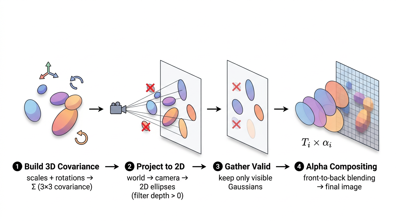
The top-level render function orchestrates these steps:

def render(means_3d, scales, rotations, colors, opacities,
           viewmat, K, H, W, bg_color=None):
    # 1. Build 3D covariance from scales and rotations
    cov3d = build_covariance_3d(scales, rotations)
 
    # 2. Project to 2D
    means_2d, cov_2d, depths, valid_mask = project_gaussians(
        means_3d, cov3d, viewmat, K, H, W
    )
 
    # 3. Gather valid properties
    valid_colors = colors[valid_mask]
    valid_opacities = opacities[valid_mask]
 
    # 4. Rasterize (alpha-composite)
    image = render_gaussians(
        means_2d, cov_2d, valid_colors, valid_opacities, depths, H, W, bg_color
    )
    return image

Let's look at each step.

Step 1: Build 3D Covariance Matrices

Each Gaussian's shape is an ellipsoid, described by a 3x3 covariance matrix. We build it from the scale and rotation parameters:

def build_covariance_3d(scales, rotations):
    R = quaternion_to_rotation_matrix(rotations)  # [N, 3, 3]
    S = torch.diag_embed(scales)                   # [N, 3, 3]
 
    M = R @ S                                      # [N, 3, 3]
    cov3d = M @ M.transpose(-1, -2)                # [N, 3, 3]
    return cov3d

The formula is $\Sigma = R S S^T R^T = M M^T$ where $M = RS$. Using $M M^T$ instead of assembling $\Sigma$ directly guarantees the result is always positive semi-definite. As we saw earlier with the broken covariance example, a negative diagonal entry would cause the Gaussian density to explode to infinity instead of fading out. This factorization makes that impossible by construction.

The quaternion_to_rotation_matrix function converts (w, x, y, z) quaternions to 3x3 rotation matrices:

def quaternion_to_rotation_matrix(q):
    w, x, y, z = q[:, 0], q[:, 1], q[:, 2], q[:, 3]
 
    R = torch.stack([
        1 - 2*y*y - 2*z*z,   2*x*y - 2*w*z,       2*x*z + 2*w*y,
        2*x*y + 2*w*z,       1 - 2*x*x - 2*z*z,   2*y*z - 2*w*x,
        2*x*z - 2*w*y,       2*y*z + 2*w*x,       1 - 2*x*x - 2*y*y,
    ], dim=-1).reshape(-1, 3, 3)
    return R

Don't worry about memorizing these expressions. This is a standard textbook formula that you can find on any quaternion reference page. In production code you'd typically use a library like scipy.spatial.transform.Rotation or pytorch3d.transforms. It's written out explicitly here so the rasterizer has zero external dependencies and every operation stays inside PyTorch's autograd graph (which is needed for backpropagation). The important thing to understand is just the input and output: 4 quaternion numbers go in, a 3x3 rotation matrix comes out. It runs on all N Gaussians simultaneously as a batched operation.

Step 2: Project Gaussians to 2D

This is the "splatting" part. We need to figure out where each 3D Gaussian lands on the 2D image plane, and what its 2D shape (footprint) looks like. This follows the EWA (Elliptical Weighted Average) splatting formulation.

Transform to camera space:

R_cam = viewmat[:3, :3]     # [3, 3] world-to-camera rotation
t_cam = viewmat[:3, 3]      # [3]    world-to-camera translation
 
means_cam = means_3d @ R_cam.T + t_cam.unsqueeze(0)  # [N, 3]

means_3d holds each Gaussian's center position in world space, a shared coordinate system where all Gaussians and all cameras coexist. means_cam is the same set of positions, but re-expressed in camera space, relative to one specific camera. Think of it as answering "from this camera's point of view, where is each Gaussian?" Instead of "5 meters north and 3 meters east" (world coordinates), it becomes "2 meters to my right and 7 meters in front of me" (camera coordinates).

The viewmat is the 4x4 world-to-camera matrix that performs this translation. R_cam (rotation) reorients the axes, and t_cam (translation) shifts the origin to the camera's position. After this transform, Gaussian centers are in camera coordinates. In this coordinate system, the camera sits at the origin looking down the +Z axis:

• +Z = forward (deeper into the scene, farther from the camera)
• +X = right
• +Y = down

So yes, Z is positive for everything the camera is looking at. An object 5 meters in front of the camera has z = 5. An object behind the camera has z < 0. This is the standard OpenCV/COLMAP camera convention.

That's why the next step uses Z as the "depth":

Cull Gaussians behind the camera:

depths = means_cam[:, 2]
valid_mask = depths > 0.2   # near plane at 0.2

means_cam[:, 2] extracts the Z component of each Gaussian's position in camera space; that's its depth. But wait, we just said +Z is everything in front of the camera. So why would any Gaussian have a negative or near-zero depth?

Because the Gaussians live in world space, spread all around the scene. A particular camera only looks in one direction. Gaussians that are behind that camera (maybe they're part of a wall the camera has its back to) will have negative Z after the world-to-camera transform. Different cameras look in different directions, so a Gaussian that's behind camera #3 might be right in front of camera #7.

To see why, picture a camera dome setup like this:

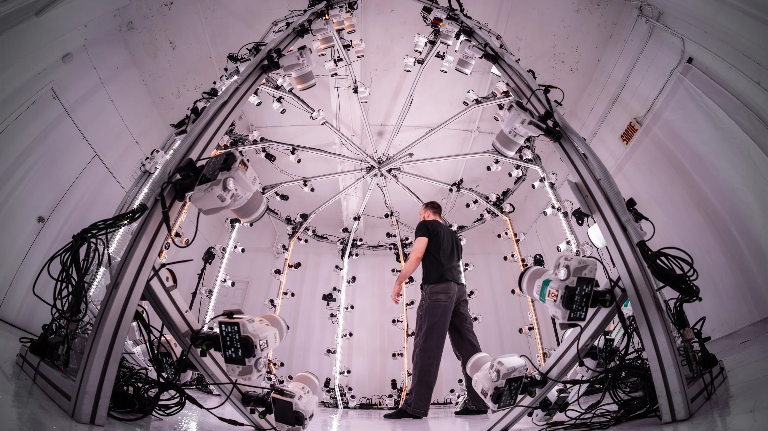
Dozens of cameras are arranged in a hemisphere, all pointing inward at the subject. Now imagine Gaussians representing the person's face, back, the floor, and the dome structure itself. A camera on the front of the dome sees the face Gaussians at positive depth (in front), but the Gaussians on the person's back have negative depth (they're behind this camera). Meanwhile, a camera on the back of the dome sees the exact opposite: back Gaussians are in front, face Gaussians are behind. Even in simpler setups (like walking around a table with your phone), you're capturing from many directions, and every viewpoint has a different set of Gaussians behind it. The depth filter ensures we only render what each camera can actually see.

The > 0.2 check also filters out Gaussians that are technically in front but extremely close. At z ≈ 0, the perspective projection divides by Z (fx * x / z), which would blow up to infinity. The 0.2 threshold acts as a near plane: anything closer than 0.2 units is discarded to avoid numerical explosions.

Perspective projection to pixel coordinates:

fx, fy = K[0, 0], K[1, 1]
cx, cy = K[0, 2], K[1, 2]
 
z = means_cam[:, 2].clamp(min=0.2)
means_2d = torch.stack([
    fx * means_cam[:, 0] / z + cx,
    fy * means_cam[:, 1] / z + cy,
], dim=-1)

This is the standard pinhole camera projection formula. The math itself isn't something you need to derive; it's the same formula used in every computer vision textbook and library. The intuition matters more:

The division by z is what creates perspective. Things farther away (large Z) get divided by a larger number, so they appear smaller on the image. Things closer (small Z) get divided by a small number, so they appear bigger. That's literally how perspective works: nearby objects look large, distant objects look small.

fx and fy (focal lengths) control how "zoomed in" the camera is: larger focal length means more zoom, so objects appear bigger.

cx and cy (the principal point) are needed because of how the coordinate systems differ. After dividing by Z, the result is centered at (0, 0), meaning a point directly in front of the camera maps to pixel (0, 0). But in an image, pixel (0, 0) is the top-left corner, not the center. If your image is 400x300, the center is around pixel (200, 150). That's roughly what cx and cy are: they shift the projection so the camera's forward axis lands at the middle of the image instead of the corner. Without this shift, everything would be offset to the top-left and the rendered image wouldn't align with the ground truth photo at all.

The output means_2d is the pixel coordinate (column, row) where each Gaussian's center lands on the image.

Project the 3D covariance to 2D using the Jacobian:

We've already projected each Gaussian's center to a 2D pixel location. But a Gaussian isn't just a point; it's a blob with a shape. We need to figure out what that 3D ellipsoid shape looks like when projected onto the 2D image. A 3D cylinder-shaped Gaussian might look like a thin line from one angle, or a circle from another.

The problem: perspective is nonlinear. The projection divides by Z ($f_x \cdot x / z$). If you push a Gaussian through a nonlinear function, the output isn't exactly a Gaussian anymore; it gets warped. The near edge (smaller $z$) gets magnified more than the far edge (larger $z$), producing a faintly egg-shaped footprint instead of a perfect ellipse.

But we can see that the warping is tiny. Consider a Gaussian centered at depth $z = 10$ with a small spread ($z = 9.5$ to $z = 10.5$). The projection rate $1/z$ varies across its extent:

• At the center ($z = 10$): rate = $0.1000$
• At the near edge ($z = 9.5$): rate = $0.1053$, just 5.3% larger
• At the far edge ($z = 10.5$): rate = $0.0952$, just 4.8% smaller

The egg is practically indistinguishable from a perfect ellipse. (For a Gaussian close to the camera, say $z = 1$ with spread $z = 0.5$ to $z = 1.5$, the rate swings from 2.0 to 0.667, much worse. But in practice, most Gaussians are small relative to their depth.)

The solution: linearize with the Jacobian. Instead of applying the true varying rate at every point, we compute the rate at the Gaussian's center and use that single fixed rate for the entire Gaussian. The center rate is 0.1000, and we pretend it's 0.1000 everywhere. This "zoom in and pretend it's linear" trick is called a first-order Taylor approximation, and the matrix of these rates is the Jacobian.

We take the projection formula from the earlier section, $(x, y, z) \to (f_x \cdot x/z + c_x, \; f_y \cdot y/z + c_y)$, and compute its partial derivatives. The Jacobian is a 2x3 matrix (2 pixel outputs, 3 camera-space inputs), where each entry answers: "if I nudge this 3D input by a tiny amount, how much does this pixel output change?"

$$J = \begin{bmatrix} f_x/z & 0 & -f_x x/z^2 \\ 0 & f_y/z & -f_y y/z^2 \end{bmatrix}$$

Each entry has a physical meaning:

• $f_x/z$: "If I nudge the point right (increase $x$), how many pixels does it shift horizontally?" At $z = 5$ with $f_x = 500$: 100 px/unit. At $z = 50$: only 10 px/unit. Farther = less movement on screen.
• $0$: Moving up in 3D doesn't affect horizontal pixel position, and vice versa. The axes are decoupled.
• $-f_x x / z^2$: "If the point moves deeper (increase $z$), does it shift horizontally?" Yes, if it's off-center. This term is directly proportional to $x$ (how far off-center the point is): a point at $x = 2$ shifts twice as much as one at $x = 1$, because it has farther to "slide" toward the center. It's inversely proportional to $z^2$: the deeper the point already is, the less additional depth matters (the convergence slows down at greater distances). And the negative sign means the shift is always toward the center: a point to the right ($x > 0$) moves left on screen, a point to the left ($x < 0$) moves right. Everything converges toward the vanishing point as it recedes.
• The second row is the same idea for the vertical pixel axis.

In code:

J = torch.zeros(M, 2, 3, device=device)
J[:, 0, 0] = fx / z
J[:, 0, 2] = -fx * means_cam[:, 0] / (z * z)
J[:, 1, 1] = fy / z
J[:, 1, 2] = -fy * means_cam[:, 1] / (z * z)

Worked example: how the Jacobian linearizes the projection. Take a Gaussian centered at $(x_0 = 1, \; y_0 = 2, \; z_0 = 10)$ with $f_x = f_y = 500$. The true projection is nonlinear: $\text{pixel}_x = 500 \cdot x / z$ and $\text{pixel}_y = 500 \cdot y / z$, where $x$, $y$, $z$ all vary across the Gaussian.

The Jacobian at the center is:

$$J = \begin{bmatrix} 50 & 0 & -5 \\ 0 & 50 & -10 \end{bmatrix}$$

(where $50 = 500/10$, $-5 = -500 \cdot 1/100$, $-10 = -500 \cdot 2/100$). Notice the $z$ column is asymmetric: $-5$ for pixel_x and $-10$ for pixel_y, because $y_0 = 2$ is farther off-center than $x_0 = 1$.

The linear approximation replaces the true nonlinear projection with a first-order Taylor expansion. The general template is:

$$f(x, y, z) \;\approx\; f(x_0, y_0, z_0) \;+\; \frac{\partial f}{\partial x} \cdot (x - x_0) \;+\; \frac{\partial f}{\partial y} \cdot (y - y_0) \;+\; \frac{\partial f}{\partial z} \cdot (z - z_0)$$

For pixel_x (first row of the Jacobian), we plug in:

• $f(x_0, y_0, z_0) = 500 \cdot 1 / 10 = 50$ (where the center lands on the image)
• $\frac{\partial f}{\partial x} = 50$ (from the Jacobian), $\frac{\partial f}{\partial y} = 0$, $\frac{\partial f}{\partial z} = -5$

$$\text{pixel}_x \;\approx\; \underbrace{50}_{\text{center}} \;+\; 50 \cdot (x - 1) \;+\; 0 \cdot (y - 2) \;+\; (-5) \cdot (z - 10)$$

For pixel_y (second row of the Jacobian):

• $f(x_0, y_0, z_0) = 500 \cdot 2 / 10 = 100$
• $\frac{\partial f}{\partial x} = 0$, $\frac{\partial f}{\partial y} = 50$, $\frac{\partial f}{\partial z} = -10$

$$\text{pixel}_y \;\approx\; \underbrace{100}_{\text{center}} \;+\; 0 \cdot (x - 1) \;+\; 50 \cdot (y - 2) \;+\; (-10) \cdot (z - 10)$$

Notice how the $y$ term contributes zero to pixel_x (moving vertically in 3D doesn't shift horizontal pixel position) but contributes 50 px/unit to pixel_y. And the depth term ($z$) pulls both pixel_x and pixel_y toward the image center as $z$ increases, but pixel_y gets pulled twice as hard ($-10$ vs $-5$) because this Gaussian is farther off-center vertically ($y_0 = 2$) than horizontally ($x_0 = 1$).

In compact form: $\text{pixel} \approx \text{pixel}_{\text{center}} + J \cdot (\mathbf{p} - \mathbf{p}_0)$. No division by $z$, just constant rates.

Let's verify at a nearby point $(1.05, \; 2.1, \; 10.2)$:

• True: pixel_x $= 500 \cdot 1.05 / 10.2 = 51.47$, pixel_y $= 500 \cdot 2.1 / 10.2 = 102.94$
• Approx: pixel_x $= 50 + 2.5 - 1.0 = 51.50$, pixel_y $= 100 + 5.0 - 2.0 = 103.00$
• Error: 0.03 and 0.06 pixels. Essentially perfect.

At a farther point $(1.5, \; 2.8, \; 11)$:

• True: pixel_x $= 68.18$, pixel_y $= 127.27$
• Approx: pixel_x $= 70.00$, pixel_y $= 130.00$
• Error: 1.82 and 2.73 pixels. Larger, but this point is far from the center where the Gaussian's density is near zero.

What the approximation actually does. The true projection rate $f_x/z$ is 52.6 at $z = 9.5$, 50.0 at $z = 10$, and 47.6 at $z = 10.5$. The Jacobian says: "I'll just use 50.0 everywhere." The near edge gets slightly too compressed, the far edge slightly too expanded. The true egg becomes a symmetric ellipse. The error is a few percent at the edges, where the Gaussian has almost no density.

While the Jacobian is fixed within a single Gaussian, it's different between Gaussians. A Gaussian at $(0, 0, 2)$ would get $f_x/z_0 = 250$ and zero cross-terms (it's on the optical axis). Every Gaussian gets its own personal Jacobian: nearby ones are in a "high magnification zone" (large 2D ellipse), far-away ones in a "low magnification zone" (tiny ellipse), off-center ones get sheared ellipses. Each Jacobian is a custom linear lens for that Gaussian's neighborhood of space.

Why linearizing unlocks the $J \Sigma J^T$ formula. There's a fundamental property: if you apply a linear transformation to a Gaussian, the result is also a Gaussian, with covariance $J \Sigma J^T$. This is the entire reason the Jacobian trick works. By replacing the nonlinear projection with a linear one, we can compute the 2D footprint as a single matrix multiply.

What if we didn't linearize? Without it, the projected shape of a 3D Gaussian through perspective wouldn't be a clean ellipse. The near edge gets magnified more than the far edge, so the shape would be slightly pear-shaped, wider on the side facing the camera, narrower on the side facing away. For a tilted ellipse, this warping would be asymmetric: one end fatter than the other. To render this exactly, you'd have to evaluate the nonlinear projection at every single pixel individually ("for this pixel, where does it land in 3D, what's the Gaussian value there?"). That's orders of magnitude slower, and you lose the elegant $T \Sigma T^T$ formula entirely. It also wouldn't be easily differentiable, which would break backpropagation.

How the Jacobian achieves the ellipse approximation: Think of the Jacobian as a snapshot of "how the projection stretches space right here, at this Gaussian's center." By multiplying the 3D covariance by this Jacobian ($J \Sigma J^T$), we're saying: "take the 3D spread of this Gaussian, and scale/shear it by however the projection distorts space at this particular location." The Jacobian translates 3D spread into 2D pixel spread. The result is always an ellipse (because a linear transform of a Gaussian is always a Gaussian), and it matches the true projected shape very closely because the Jacobian is evaluated right at the center where the Gaussian has most of its mass.

In short: the Jacobian is the bridge between "3D ellipsoid shape" and "2D ellipse on screen." It encodes how perspective distorts space at each Gaussian's location, and the $T \Sigma T^T$ formula uses that to warp the 3D covariance into the correct 2D footprint: cheaply, differentiably, and as a simple matrix multiply.

The trade-off: accept a tiny approximation error (a few percent at the edges) and in return get a simple, fast, differentiable formula.

The code that computes the 2D covariance:

W = R_cam.unsqueeze(0).expand(M, -1, -1)   # [M, 3, 3]
T = J @ W                                    # [M, 2, 3]
cov_2d = T @ cov3d_valid @ T.transpose(-1, -2)  # [M, 2, 2]

This combines two stages into one. The 3D covariance is in world space, but the Jacobian expects camera space. So we first rotate by $R_{\text{cam}}$ (world → camera), then project with $J$ (camera 3D → image 2D). Combined: $T = J \cdot R_{\text{cam}}$, and $\Sigma_{2D} = T \cdot \Sigma \cdot T^T$.

The result cov_2d is a 2x2 matrix per Gaussian, an ellipse on the image plane.

Numerical example of the full $J \Sigma J^T$ multiply. Take a spherical Gaussian at depth z = 5, with fx = fy = 500, centered on the optical axis (x = 0, y = 0):

$$J = \begin{bmatrix} 100 & 0 & 0 \\ 0 & 100 & 0 \end{bmatrix}$$

If the 3D covariance is $\Sigma = 0.01 \cdot I$ (a small sphere):

$$\Sigma_{2D} = J \cdot \Sigma \cdot J^T = \begin{bmatrix} 100 & 0 & 0 \\ 0 & 100 & 0 \end{bmatrix} \begin{bmatrix} 0.01 & 0 & 0 \\ 0 & 0.01 & 0 \\ 0 & 0 & 0.01 \end{bmatrix} \begin{bmatrix} 100 & 0 \\ 0 & 100 \\ 0 & 0 \end{bmatrix} = \begin{bmatrix} 100 & 0 \\ 0 & 100 \end{bmatrix}$$

The diagonal entries (100, 100) are variances in squared pixel units. The actual spread (standard deviation) is $\sqrt{100} = 10$ pixels. At 3 standard deviations (where the code draws the boundary), this Gaussian covers a circle about 30 pixels across.

If the same Gaussian were at z = 50 (10x farther), the Jacobian entries would be 10x smaller (fx/z = 500/50 = 10), and the covariance would be 100x smaller (because covariance goes through $J \Sigma J^T$, so a 10x smaller J means the covariance shrinks by $10 \times 10 = 100$). The standard deviation would be $\sqrt{1} = 1$ pixel, so it'd cover only about 1 pixel on screen. Farther away = smaller on screen, exactly as you'd expect from perspective.

Adding numerical padding:

cov_2d[:, 0, 0] += 0.3
cov_2d[:, 1, 1] += 0.3

This adds 0.3 to the diagonal of every 2D covariance for two reasons:

1. Preventing division by zero. Later we invert this 2x2 matrix ($\Sigma_{2D}^{-1}$). If a Gaussian projects to an almost zero-area footprint (a cylinder viewed end-on is a dot), the determinant would be near zero and the inverse would blow up. The padding ensures every Gaussian covers at least a small area.
2. Anti-aliasing. A very distant or small Gaussian might be thinner than a single pixel, causing it to flicker as the camera moves. The 0.3 padding guarantees every Gaussian covers at least a fraction of a pixel, producing smoother renders.

Step 3: Alpha Compositing

Now we have N sorted 2D Gaussians and need to produce an image. The render_gaussians function does this.

Sort front-to-back by depth:

sort_idx = torch.argsort(depths)
means_2d = means_2d[sort_idx]
# ... same for cov_2d, colors, opacities

Sorting is essential for correct alpha compositing. Closer Gaussians occlude farther ones.

Pre-compute the inverse of each 2D covariance:

a = cov_2d[:, 0, 0]; b = cov_2d[:, 0, 1]
c = cov_2d[:, 1, 0]; d = cov_2d[:, 1, 1]
det = (a * d - b * c).clamp(min=1e-6)
 
inv_a =  d / det
inv_b = -b / det
inv_c = -c / det
inv_d =  a / det

We need the inverse to evaluate the Gaussian density at each pixel. Since these are 2x2 matrices, the inverse is computed analytically (much faster than a general matrix inverse).

Compute a bounding radius for each Gaussian:

Before we evaluate every Gaussian at every pixel (which would be very expensive), we want to know: "how far from its center does each Gaussian actually matter?" A tight, small Gaussian only affects pixels within a few pixels of its center. A big, spread-out one affects pixels much farther away. If we know the maximum radius of influence, we can skip all pixels outside it.

The 2D covariance matrix tells us the Gaussian's spread, but it might be an ellipse (stretched more in one direction than another). We need the longest direction, the semi-major axis, to get a safe bounding circle that contains the entire ellipse.

trace = a + d
disc = (trace * trace - 4 * det).clamp(min=0)
lambda_max = 0.5 * (trace + torch.sqrt(disc))
radius = torch.ceil(3.0 * torch.sqrt(lambda_max))

Line by line:

trace = a + d: the trace of the 2x2 covariance matrix (sum of diagonal entries). For $\begin{bmatrix} a & b \\ c & d \end{bmatrix}$, the trace is $a + d$.

Why does this equal the sum of the eigenvalues? Let's derive it. Eigenvalues $\lambda$ of a matrix $M$ satisfy $\det(M - \lambda I) = 0$. For our 2x2 covariance:

$$\det\begin{pmatrix} a - \lambda & b \\ c & d - \lambda \end{pmatrix} = (a - \lambda)(d - \lambda) - bc = 0$$

Expanding:

$$\lambda^2 - (a + d)\lambda + (ad - bc) = 0$$

That's $\lambda^2 - \text{trace} \cdot \lambda + \text{det} = 0$, a quadratic in $\lambda$. The two roots $\lambda_1, \lambda_2$ are the eigenvalues. By the quadratic formula:

$$\lambda = \frac{\text{trace} \pm \sqrt{\text{trace}^2 - 4 \cdot \text{det}}}{2}$$

This is exactly what the next two lines of code compute. The trace and determinant are all we need to find both eigenvalues; they're just the coefficients of the quadratic. The $+$ branch gives the larger eigenvalue (the direction of maximum spread), which is the one we care about for the bounding radius.

What's the significance? The eigenvalues of the covariance matrix are the variances along the ellipse's two principal axes. If the 2D covariance has eigenvalues 100 and 25, it means the Gaussian spreads with variance 100 along its widest direction and variance 25 along the narrow direction (standard deviations of 10 and 5 pixels). The trace (125 = 100 + 25) captures the "total spread" of the Gaussian. We don't actually need the trace by itself; we need it as an intermediate step to compute the individual eigenvalues using the quadratic formula in the next line.

disc = (trace * trace - 4 * det).clamp(min=0): the discriminant of the characteristic equation. The eigenvalues of a 2x2 matrix are the roots of $\lambda^2 - \text{trace} \cdot \lambda + \text{det} = 0$, which by the quadratic formula gives $\lambda = \frac{\text{trace} \pm \sqrt{\text{trace}^2 - 4 \cdot \text{det}}}{2}$. This line computes the part under the square root. The .clamp(min=0) prevents negative values from floating-point rounding errors (the discriminant should theoretically always be non-negative for a valid covariance matrix).

lambda_max = 0.5 * (trace + torch.sqrt(disc)): the larger eigenvalue (using the $+$ branch of the $\pm$). This is the variance along the direction where the Gaussian spreads the most. For example, if the ellipse is 20 pixels wide and 5 pixels tall, $\lambda_{\max}$ corresponds to the 20-pixel direction.

radius = torch.ceil(3.0 * torch.sqrt(lambda_max)): convert the largest variance to a pixel radius.

Recall that our 2D covariance is in pixel-space (we already projected from 3D to pixel coordinates earlier). So $\lambda_{\max}$ is a variance measured in pixels-squared. Taking the square root gives the standard deviation, which is in plain pixels. If $\lambda_{\max} = 100$, the standard deviation is $\sqrt{100} = 10$ pixels, meaning the Gaussian's density drops to about 60% of its peak at 10 pixels from center along the widest direction.

Multiplying by 3.0 gives 3 standard deviations ($3 \times 10 = 30$ pixels). Why 3? For a Gaussian, 99.7% of its density falls within 3 standard deviations. At that distance, the density has dropped to $\exp(-0.5 \times 3^2) = \exp(-4.5) \approx 0.011$, about 1% of the peak. Anything beyond this contributes essentially nothing to the pixel color, so it's safe to skip.

torch.ceil rounds up to the next whole pixel so we don't accidentally clip the edge (29.3 becomes 30, not 29).

For example, if the 2D covariance has eigenvalues 100 and 25 (an ellipse 10px by 5px in standard deviation), then $\lambda_{\max} = 100$, $\sqrt{100} = 10$, and the radius is $\lceil 3 \times 10 \rceil = 30$ pixels. Any pixel more than 30 pixels from this Gaussian's center can be safely skipped.

This radius tensor (one value per Gaussian) doesn't get used immediately; it gets used during chunk processing below. When we process a chunk of pixels, we ask: "is the distance from this Gaussian's center to the chunk's center less than radius + chunk_radius?" That radius here is exactly the per-Gaussian bounding radius we just computed. So the eigenvalue computation feeds directly into the culling that makes chunk processing fast.

Create a pixel grid:

ys = torch.arange(H, device=device, dtype=torch.float32) + 0.5
xs = torch.arange(W, device=device, dtype=torch.float32) + 0.5
grid_y, grid_x = torch.meshgrid(ys, xs, indexing='ij')
pixels = torch.stack([grid_x.reshape(-1), grid_y.reshape(-1)], dim=-1)

Think of an image as a grid of little squares, not a grid of points. Pixel 0 isn't a dot at position 0; it's a square that covers the area from 0.0 to 1.0. The "color" of that pixel should be evaluated at its center, which is 0.5. Pixel 1 covers 1.0 to 2.0, center at 1.5. And so on.

Without the + 0.5, torch.arange(W) gives [0, 1, 2, ...], the left edges of each pixel. Adding 0.5 shifts to [0.5, 1.5, 2.5, ...], the centers. This matters because when we compute the distance from a pixel to a Gaussian's center, we want the distance to the middle of the pixel, not its corner. Using corner positions would introduce a systematic half-pixel offset, making the rendered image slightly shifted compared to the ground truth.

torch.meshgrid then creates every (x, y) combination to cover the full image: for a 400x300 image, that's 120,000 pixel-center coordinates. pixels is the flattened list of all these coordinates, shape [H*W, 2].

Process pixels in chunks to keep GPU memory bounded:

CHUNK_SIZE = 2048
for chunk_start in range(0, total_pixels, CHUNK_SIZE):
    chunk_px = pixels[chunk_start:chunk_end]

The pixels array is a flat list of all pixel coordinates, ordered row by row (because meshgrid with indexing='ij' produces row-major order, and we reshaped to 1D). So the first W entries are row 0 (left to right), the next W entries are row 1, and so on. Each chunk is a contiguous slice of 2,048 pixels from this list. For a 400-pixel-wide image, one chunk covers about 5 full rows (2048 / 400 ≈ 5), a horizontal band of the image.

This spatial grouping matters. The code uses it for a second round of culling. Recall that we already did one round earlier: the depth culling in project_gaussians (depths > 0.2) removed all Gaussians behind the camera or too close. That was a coarse, global filter. What remains are Gaussians that are somewhere in front of the camera, but most of them are far from any given pixel strip. This chunk culling is finer-grained: for each chunk, it computes the bounding box of all pixels in the chunk (chunk_center_x, chunk_center_y, chunk_radius), then checks which of the surviving Gaussians are close enough to possibly overlap that region:

chunk_center_x = (chunk_px[:, 0].min() + chunk_px[:, 0].max()) / 2
chunk_center_y = (chunk_px[:, 1].min() + chunk_px[:, 1].max()) / 2
chunk_radius = max(
    (chunk_px[:, 0].max() - chunk_px[:, 0].min()) / 2,
    (chunk_px[:, 1].max() - chunk_px[:, 1].min()) / 2,
) + 1
dist_to_chunk = torch.sqrt(
    (means_2d[:, 0] - chunk_center_x) ** 2 +
    (means_2d[:, 1] - chunk_center_y) ** 2
)
active = dist_to_chunk < (radius + chunk_radius)

This asks: "is the distance from each Gaussian's center to the chunk's center less than the sum of the Gaussian's radius and the chunk's chunk_radius?" Here, radius is the per-Gaussian bounding radius we computed earlier from the eigenvalues of the 2D covariance (the 3 * sqrt(lambda_max) value). A Gaussian with a small, tight 2D projection has a small radius and is easy to cull. A big, spread-out Gaussian has a large radius and stays active for more chunks. This is where all the eigenvalue math pays off: it tells us exactly how far each Gaussian reaches in pixel space. Only Gaussians that pass this test are evaluated for the chunk. If a chunk covers rows 50-70 and a Gaussian is centered at row 250, it's far outside and gets skipped entirely. This is a huge speedup: instead of evaluating all N Gaussians for all pixels, each chunk only processes the handful of Gaussians that actually overlap its region.

The chunk size also controls memory. For each chunk, the code creates a [chunk_size, N_active] tensor (distance from every pixel in the chunk to every active Gaussian). Processing all 120,000 pixels at once with 5,000 Gaussians would need a 120,000 x 5,000 tensor (~10 GB). Processing 2,048 at a time with maybe 500 active Gaussians per chunk keeps it to ~4 MB, very manageable.

This culling is effective, but the geometry of our row-wise strips limits how tight it can be. Our chunks are ~400px wide and ~5px tall, so the bounding circle has chunk_radius = 201, nearly the entire image width. That means a Gaussian passes the culling test even if it's hundreds of pixels away from the strip, as long as it's within 201px of the chunk center. Production rasterizers avoid this problem entirely by using square 2D tiles instead of wide strips. The diagram below visualizes the full pipeline, from eigenvalue-based radius computation through the circle-circle culling test, and shows why the chunk shape matters so much.

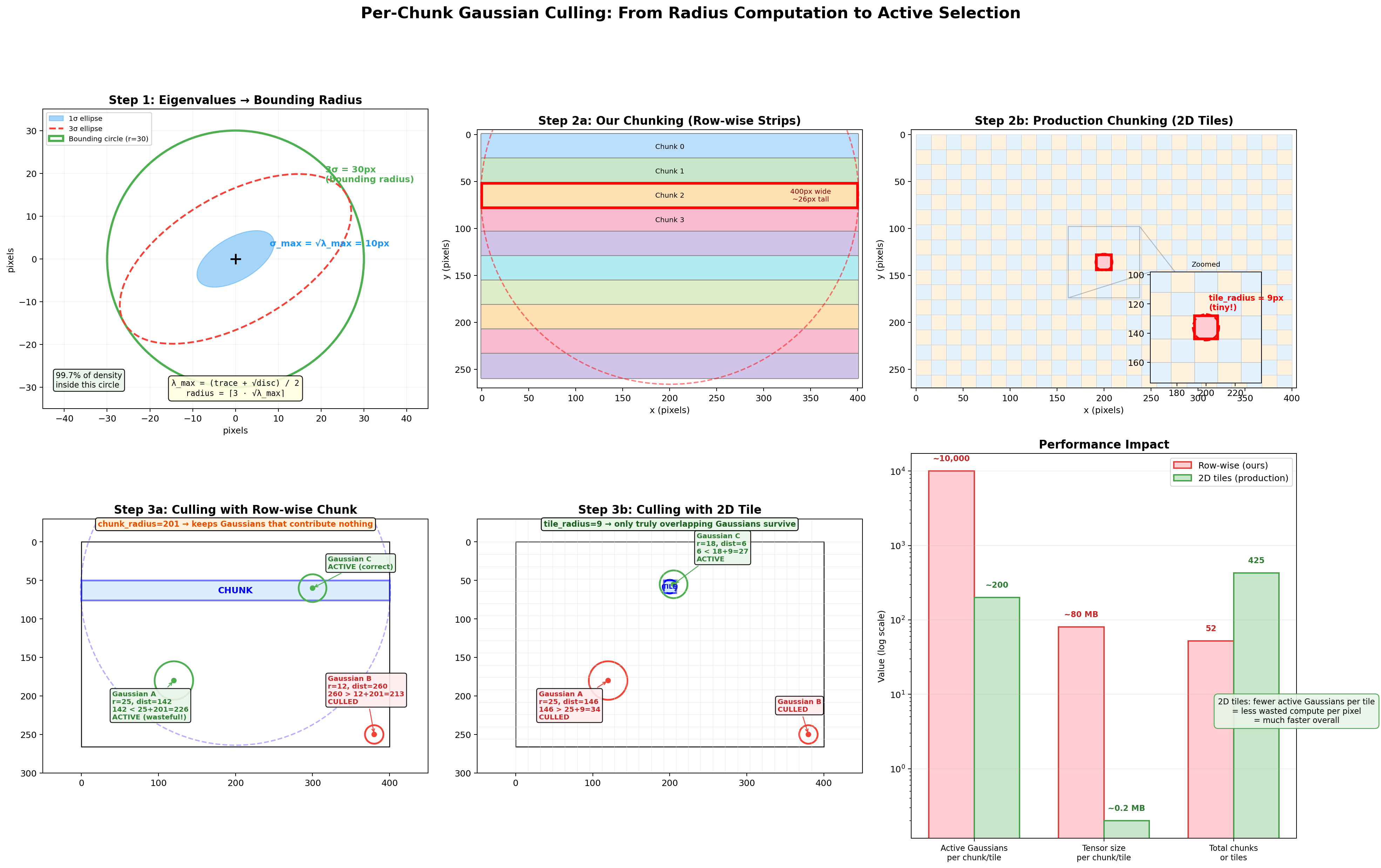
The six panels follow the data flow left-to-right, top-to-bottom:

Step 1: Eigenvalues to Bounding Radius (top-left). A single Gaussian's 2D covariance on the image plane. The solid blue ellipse is the 1-sigma contour (density above ~60% of peak), the dashed red ellipse is the 3-sigma contour (density at ~1%), and the green circle is the bounding radius we compute: radius = ceil(3 * sqrt(lambda_max)). It's a circle rather than an ellipse because we use only the largest eigenvalue, which is conservative but guaranteed to contain the full 3-sigma ellipse in every direction.

Step 2a: Row-wise Strip Layout (top-center). Our 400x266 image divided into horizontal strip chunks. Each strip spans the full image width (~400px) but only ~5 rows tall. The red-highlighted chunk shows its bounding circle: chunk_radius = max(400/2, 5/2) + 1 = 201px. That circle extends far above and below the actual strip, the root cause of the culling inefficiency.

Step 2b: 2D Tile Layout (top-right). The same image divided into 16x16 production-style tiles (as used in the original CUDA rasterizer from Kerbl et al.). The zoomed inset shows a single tile's bounding circle: tile_radius = max(16/2, 16/2) + 1 = 9px. The circle barely extends beyond the tile's edges, making the culling test dist < radius[j] + tile_radius far more selective.

Step 3a: Culling with Row-wise Chunk (bottom-left). Three Gaussians tested against the blue strip. Gaussian A is 165px from the chunk center (far from any pixel in the strip) but passes because 165 < 25 + 201 = 226. It's marked ACTIVE despite contributing nothing: wasted work. Gaussian B is far enough to be culled. Gaussian C correctly survives. The huge chunk_radius keeps Gaussians that don't actually overlap the strip.

Step 3b: Culling with 2D Tile (bottom-center). The same three Gaussians tested against a 16x16 tile. Now Gaussian A fails: 165 > 25 + 9 = 34. Only Gaussian C, which genuinely overlaps the tile, survives. The tight tile_radius = 9 is far more discriminating.

Performance Impact (bottom-right). Row-wise strips keep ~10,000 active Gaussians per chunk and ~80 MB of intermediate tensors. 2D tiles keep ~200 per tile and ~0.2 MB. Row-wise has fewer total chunks (52 vs 425 tiles), but each chunk does far more work because it can't cull effectively. The net result: 2D tiling processes roughly 50x fewer Gaussian-pixel pairs across the full image.

Why do we use row-wise strips anyway? They're simpler to implement in pure PyTorch. 2D tiling requires a binning pass (assign each Gaussian to the tiles it overlaps), per-tile Gaussian lists of variable length, and per-tile depth sorting, operations that are natural in CUDA but awkward without custom ops. Row-wise strips let us use simple contiguous slicing (pixels[start:end]) and still get meaningful culling. For an educational implementation, that tradeoff is worth it.

Gather only the active Gaussians for this chunk:

After culling, the code extracts only the surviving Gaussians' data so that all subsequent work operates on the small active subset instead of all N Gaussians:

a_means = means_2d[active_idx]
a_inv_a = inv_a[active_idx]
a_inv_b = inv_b[active_idx]
a_inv_c = inv_c[active_idx]
a_inv_d = inv_d[active_idx]
a_colors = colors[active_idx]
a_opacities = opacities[active_idx]

The a_ prefix stands for "active." active_idx is the list of Gaussian indices that passed the culling test above. So a_opacities contains only the opacities of the, say, 500 Gaussians (out of 5,000 total) that are close enough to this chunk to matter. Same for a_means (their 2D centers), a_inv_a/b/c/d (their inverse covariance entries), and a_colors (their RGB values). Everything from here on in the chunk loop works with these smaller [Na]-sized tensors instead of the full [N]-sized ones.

To trace where a_opacities ultimately comes from: the GaussianModel stores a raw parameter _opacities_raw, initialized to 0.0 for every Gaussian. The activated opacity is sigmoid(_opacities_raw), so every Gaussian starts at sigmoid(0) = 0.5 (50% transparent). During training, gradients push these raw values up or down. Gaussians that the scene needs become nearly opaque (raw goes to large positive values, sigmoid approaches 1.0), while useless ones fade away (raw goes negative, sigmoid approaches 0.0) and eventually get pruned. By the time opacities reaches this line, it's already been through sigmoid and is in [0, 1]. The [active_idx] indexing just selects the subset relevant to this chunk.

Evaluate the Gaussian density at each pixel:

The core question at this stage is: for every pixel in the chunk and every active Gaussian, how much does that Gaussian contribute to that pixel's color? A Gaussian centered right on a pixel contributes a lot. A Gaussian centered far away contributes almost nothing. But "far" isn't just about Euclidean distance; it depends on the Gaussian's shape. If a Gaussian is a wide horizontal ellipse, a pixel 20px to the right might still be "close" (inside the ellipse), while a pixel 10px above might be "far" (outside the narrow axis). The Mahalanobis distance handles this: it's a shape-aware distance that stretches and squishes space according to the Gaussian's covariance, so that "1 unit of Mahalanobis distance" always means "1 standard deviation away," regardless of direction.

Concretely: imagine a Gaussian centered at pixel (200, 150) that's an ellipse stretched 20px wide and 5px tall. A pixel at (210, 150) is 10px to the right, which is only 0.5 standard deviations along the wide axis, so the Mahalanobis distance is small and the Gaussian contributes strongly. A pixel at (200, 160) is 10px below, which is 2 standard deviations along the narrow axis, so the Mahalanobis distance is large and the contribution drops off steeply. Euclidean distance treats both as "10 pixels away." Mahalanobis distance knows one is close and the other is far, because it accounts for the elliptical shape.

The formula for a 2D Gaussian's density at pixel position $p$ is:

$$G(p) = \exp\left(-\frac{1}{2} \, (p - \mu)^T \, \Sigma^{-1} \, (p - \mu)\right)$$

where $\mu$ is the Gaussian's 2D center, $\Sigma$ is the 2D covariance matrix, and $(p - \mu)$ is the offset vector from the center to the pixel. The quantity $(p - \mu)^T \Sigma^{-1} (p - \mu)$ is the squared Mahalanobis distance. If we let $d = (dx, dy) = p - \mu$ and write the inverse covariance as $\Sigma^{-1} = \begin{bmatrix} A & B \\ C & D \end{bmatrix}$, then expanding the matrix multiply step by step:

First, compute $\Sigma^{-1} d$ (matrix times column vector):

$$\Sigma^{-1} d = \begin{bmatrix} A & B \\ C & D \end{bmatrix} \begin{bmatrix} dx \\ dy \end{bmatrix} = \begin{bmatrix} A \cdot dx + B \cdot dy \\ C \cdot dx + D \cdot dy \end{bmatrix}$$

Then, compute $d^T$ times that result (row vector times column vector, giving a scalar):

$$d^T \cdot (\Sigma^{-1} d) = \begin{bmatrix} dx & dy \end{bmatrix} \begin{bmatrix} A \cdot dx + B \cdot dy \\ C \cdot dx + D \cdot dy \end{bmatrix}$$

$$= dx \cdot (A \cdot dx + B \cdot dy) + dy \cdot (C \cdot dx + D \cdot dy)$$

$$= A \cdot dx^2 + B \cdot dx \cdot dy + C \cdot dx \cdot dy + D \cdot dy^2$$

$$= A \cdot dx^2 + (B + C) \cdot dx \cdot dy + D \cdot dy^2$$

The two middle terms ($B \cdot dx \cdot dy$ and $C \cdot dx \cdot dy$) both multiply $dx \cdot dy$, so they combine into $(B + C) \cdot dx \cdot dy$. That's why the code adds a_inv_b + a_inv_c together as a single coefficient for the cross-term.

This is exactly what the code computes:

dx = chunk_px[:, 0:1] - a_means[:, 0].unsqueeze(0)  # [C, Na]
dy = chunk_px[:, 1:2] - a_means[:, 1].unsqueeze(0)  # [C, Na]
 
power = -0.5 * (
    a_inv_a.unsqueeze(0) * dx * dx +
    (a_inv_b + a_inv_c).unsqueeze(0) * dx * dy +
    a_inv_d.unsqueeze(0) * dy * dy
)
 
gauss = torch.exp(power.clamp(min=-16.0))

Line by line:

dx = chunk_px[:, 0:1] - a_means[:, 0].unsqueeze(0): for every pixel in the chunk and every active Gaussian, compute the horizontal offset. chunk_px has shape [C, 2] (C pixels, each with x and y), and a_means has shape [Na, 2] (Na active Gaussians). The [:, 0:1] grabs the x-coordinates as a column vector [C, 1], and .unsqueeze(0) makes the Gaussian centers [1, Na]. Broadcasting gives a [C, Na] tensor: every pixel's x minus every Gaussian's x. For example, if pixel 7 is at x=350.5 and Gaussian 3 is centered at x=200, then dx[7, 3] = 150.5.

dy = chunk_px[:, 1:2] - a_means[:, 1].unsqueeze(0): same thing for the vertical offset. dy[7, 3] is the vertical distance from pixel 7 to Gaussian 3.

power = -0.5 * (A * dx² + (B+C) * dx*dy + D * dy²): this is the exponent of the Gaussian formula, which is $-\frac{1}{2}$ times the squared Mahalanobis distance. Each term corresponds to one part of the matrix multiply $d^T \Sigma^{-1} d$:

• a_inv_a * dx * dx is the $A \cdot dx^2$ term, how much the horizontal offset contributes. If the Gaussian is narrow horizontally, $A$ is large (the inverse covariance penalizes horizontal distance heavily), so even a small dx produces a large penalty.
• (a_inv_b + a_inv_c) * dx * dy is the $(B+C) \cdot dx \cdot dy$ cross-term. This captures the ellipse's tilt. If the Gaussian is axis-aligned, this is zero. If the ellipse is tilted at 45°, this is nonzero and mixes horizontal and vertical offsets.
• a_inv_d * dy * dy is the $D \cdot dy^2$ term, how much the vertical offset contributes.

The .unsqueeze(0) on the inverse covariance values broadcasts them from [Na] to [1, Na], so the same inverse covariance applies to all pixels for a given Gaussian.

gauss = torch.exp(power.clamp(min=-16.0)): convert the exponent to actual Gaussian density. When power is 0 (pixel is exactly at the Gaussian center), exp(0) = 1.0, maximum contribution. When power is -2 (about 2 standard deviations away), exp(-2) ≈ 0.14, 14% contribution. When power is -8 (about 4 standard deviations), exp(-8) ≈ 0.0003, essentially zero. The .clamp(min=-16.0) caps the exponent so that exp(-16) ≈ 1.1e-7 is the smallest value, preventing floating-point underflow to exactly zero (which could cause numerical issues in downstream gradients).

A worked example: suppose a Gaussian is centered at (200, 150) with a 2D covariance whose inverse is $\Sigma^{-1} = \begin{bmatrix} 0.01 & 0 \\ 0 & 0.16 \end{bmatrix}$ (a wide horizontal ellipse: small $A$ means lenient horizontally, large $D$ means strict vertically). For a pixel at (210, 150): $dx=10, dy=0$, so $\text{power} = -0.5 \times (0.01 \times 100 + 0 + 0) = -0.5$, giving $\exp(-0.5) = 0.61$, a strong contribution. For a pixel at (200, 160): $dx=0, dy=10$, so $\text{power} = -0.5 \times (0 + 0 + 0.16 \times 100) = -8.0$, giving $\exp(-8) = 0.0003$, virtually nothing. Same 10-pixel Euclidean distance, but the Mahalanobis distance correctly reflects the elliptical shape.

Compute alpha and composite front-to-back:

Think of looking through a stack of colored glass panes, sorted from nearest to farthest. The first pane blocks some light and contributes its color. Whatever light passes through reaches the second pane, which blocks some more and adds its own color. And so on. Each Gaussian is one such pane.

alpha = (a_opacities.unsqueeze(0) * gauss).clamp(max=0.99)

alpha is the effective opacity of each Gaussian at each pixel, meaning how much of a "blocker" it is at that specific location. It's the product of two things:

• a_opacities: the Gaussian's intrinsic opacity (how opaque it is in general; a dense surface Gaussian might be 0.95, a wispy fog Gaussian might be 0.1).
• gauss: the Gaussian density at this pixel (how close the pixel is to the Gaussian's center, accounting for elliptical shape; 1.0 at the center, fading to ~0 far away).

The product means: a Gaussian that's intrinsically very opaque (0.95) but whose center is far from this pixel (gauss = 0.01) has a tiny effective alpha at this pixel ($0.95 \times 0.01 = 0.0095$). A Gaussian that's moderately opaque (0.6) and centered right on this pixel (gauss = 0.9) has a strong alpha ($0.6 \times 0.9 = 0.54$). The .clamp(max=0.99) prevents any single Gaussian from being fully opaque, ensuring Gaussians behind it can still contribute a little.

one_minus_alpha = 1.0 - alpha
T = torch.cat([
    torch.ones(C, 1, device=device),
    torch.cumprod(one_minus_alpha[:, :-1], dim=1)
], dim=1)

1 - alpha is how much light each Gaussian lets through. If alpha is 0.7 (blocks 70%), then 1 - alpha = 0.3 (lets 30% through).

T is the transmittance: for each Gaussian, what fraction of light actually reaches it after passing through all the Gaussians in front. This is computed as the cumulative product of all the (1 - alpha) values of the Gaussians ahead of it in the depth order.

Concrete example with 3 Gaussians at one pixel, sorted front-to-back:

The first Gaussian always gets $T = 1$ (torch.ones(C, 1, ...); nothing is in front). For G2, $T = (1 - 0.7) = 0.3$. For G3, $T = (1 - 0.7) \times (1 - 0.5) = 0.3 \times 0.5 = 0.15$. That's exactly what cumprod(one_minus_alpha[:, :-1]) computes: the running product of pass-through fractions, shifted by one position so each Gaussian sees the product of everything before it.

Why [:, :-1] (drop the last element)? Because transmittance $T_i$ is the product of $(1 - \alpha_j)$ for all Gaussians before $i$, not including $i$ itself. If you did cumprod on all Na elements, each result would include that Gaussian's own $(1 - \alpha)$, and everything would be shifted one step forward from what we need. By doing cumprod on the first Na-1 elements (dropping the last), we get Na-1 values, then prepend a 1.0 for the first Gaussian, giving exactly Na transmittance values that line up correctly:

• [1.0, cumprod₀, cumprod₁] = [1.0, (1-α₀), (1-α₀)(1-α₁)] = [T₀, T₁, T₂]

If we hadn't dropped the last element, we'd have Na+1 values after prepending the 1.0, which wouldn't match the Na Gaussians.

weights = T * alpha
chunk_rendered = weights @ a_colors

weights = T * alpha combines both factors: how much light reaches this Gaussian ($T$) and how much of that light it absorbs ($\alpha$). Continuing our example:

If G1 is red (1, 0, 0), G2 is green (0, 1, 0), and G3 is blue (0, 0, 1), the final pixel color is:

$$C = 0.70 \times (1,0,0) + 0.15 \times (0,1,0) + 0.12 \times (0,0,1) = (0.70, 0.15, 0.12)$$

The pixel is mostly red (the nearest Gaussian dominates), with a bit of green and a trace of blue showing through. The weights sum to $0.70 + 0.15 + 0.12 = 0.97$, leaving 3% for the background color (which gets blended in next).

This is the volume rendering equation in discrete form:

$$C = \sum_i T_i \cdot \alpha_i \cdot c_i \quad \text{where} \quad T_i = \prod_{j < i} (1 - \alpha_j)$$

The matrix multiply weights @ a_colors is a compact way of computing this weighted color sum across all Gaussians for each pixel simultaneously. weights has shape [C, Na] (one weight per pixel-Gaussian pair) and a_colors has shape [Na, 3] (RGB per Gaussian), so the result is [C, 3], an RGB color for every pixel in the chunk.

Finally, the remaining transmittance is used to blend in the background color:

remaining_T = T[:, -1:] * one_minus_alpha[:, -1:]
chunk_rendered = chunk_rendered + remaining_T * bg_color.unsqueeze(0)

After all Gaussians have been composited, some light might still be left over; it passed through every single Gaussian without being fully absorbed. That leftover light should show the background color. T[:, -1:] is the transmittance of the last Gaussian (how much light reached it). one_minus_alpha[:, -1:] is how much of that light the last Gaussian let through. Their product is the fraction of light that made it past everything:

$$T_\text{remaining} = T_\text{last} \times (1 - \alpha_\text{last})$$

Continuing our example: $T_2 = 0.15$, $\alpha_2 = 0.8$, so $T_\text{remaining} = 0.15 \times 0.2 = 0.03$. That 3% of light shows the background color. If the background is white (1, 1, 1), it adds $0.03 \times (1, 1, 1) = (0.03, 0.03, 0.03)$ to the pixel, making the final color $(0.70, 0.15, 0.12) + (0.03, 0.03, 0.03) = (0.73, 0.18, 0.15)$. Now the weights sum to exactly 1.0: $0.70 + 0.15 + 0.12 + 0.03 = 1.0$.

The [:, -1:] (with the colon after -1) instead of [:, -1] keeps the tensor 2D rather than collapsing a dimension, so broadcasting with bg_color works correctly.

Assembling the full image:

After each chunk computes its pixel colors, it writes them into a pre-allocated flat tensor:

rendered[chunk_start:chunk_end] = chunk_rendered

rendered is created as torch.zeros(total_pixels, 3) before the chunk loop starts, one RGB slot per pixel, all black. Each chunk fills in its slice. After the loop finishes, the flat tensor is reshaped back into an image:

return rendered.reshape(H, W, 3)

There's no separate "merge" or "stitch" step. The chunks are independent because each pixel belongs to exactly one chunk, and the Gaussians are already sorted globally by depth before the loop begins. So each chunk can composite front-to-back for its own pixels without knowing anything about the other chunks. This isn't a simplification we made; chunks/tiles are independent in production code too. The 16×16 tiles from the original paper (which we compared against our row-wise strips in the culling diagram above) work the same way: each tile independently composites its assigned Gaussians front-to-back. Tiles never need to communicate, which is exactly what makes the algorithm so parallelizable on GPUs.

The final [H, W, 3] tensor is the rendered image, ready to be compared against the ground-truth photograph in the loss function.

The Loss Function: L1 + SSIM

The loss function compares the rendered image to the ground-truth photograph. The code uses a weighted combination of two losses:

l1_loss = F.l1_loss(rendered, gt_image)
 
rendered_bchw = rendered.permute(2, 0, 1).unsqueeze(0)
gt_bchw = gt_image.permute(2, 0, 1).unsqueeze(0)
ssim_val = compute_ssim(rendered_bchw, gt_bchw)
ssim_loss = 1.0 - ssim_val
 
loss = (1 - lambda_ssim) * l1_loss + lambda_ssim * ssim_loss

L1 loss (mean absolute error) measures per-pixel difference. If a pixel is red but should be green, the loss is proportional to the color difference.

SSIM loss (Structural Similarity) captures something L1 misses: structural relationships between neighboring pixels. L1 treats every pixel independently; it only cares "is this pixel the right color?" But images aren't random collections of pixels. A sharp edge means a bright pixel next to a dark pixel. A texture means a repeating pattern across neighboring pixels. A blurry image might have nearly the same average color as the sharp original (low L1 error) but look terrible because all edges and textures are smeared out. SSIM catches this by comparing patches of pixels rather than individual ones.

The intuition: SSIM slides a small window (11×11 pixels) across both images. At each position, it asks three questions about the patch:

1. Luminance: are the two patches roughly the same brightness? (compares local means)
2. Contrast: do the two patches have similar variation? (compares local variances)
3. Structure: do bright and dark pixels fall in the same places? (compares correlation)

If the rendered image has an edge where the ground truth has an edge, all three scores are high. If the rendered image is blurry where the ground truth is sharp, the contrast and structure scores drop.

SSIM is a well-known image quality metric; you don't need to implement it yourself. Standard libraries like torchmetrics.StructuralSimilarityIndexMeasure or pytorch_msssim.ssim provide it out of the box. This codebase includes its own implementation to avoid the extra dependency, but any standard SSIM function works.

The SSIM score ranges from 0 to 1 (1.0 = identical images). The loss used in training is 1 - ssim_val, so a perfect match gives zero loss. The default weight is lambda_ssim = 0.2, meaning the combined loss is 80% L1 and 20% SSIM. L1 does the heavy lifting of getting each pixel's color right, while SSIM adds a nudge toward preserving sharp edges and textures rather than blurring them out.

The Backward Pass: How Gradients Flow

There are no hand-written backward passes here. Every operation in the forward pass (build_covariance_3d, project_gaussians, the alpha compositing loop) uses standard PyTorch operations (torch.exp, torch.sigmoid, matrix multiplies, etc.). So loss.backward() just works. PyTorch's autograd walks back through the entire chain and computes gradients for every learnable parameter automatically.

optimizer.zero_grad()
loss.backward()
 
model.update_grad_stats()   # accumulate gradient info for densification
 
optimizer.step()

Tracing the gradient chain backward from the loss:

1. The loss says "these pixels are too red" → gradients on the rendered pixel colors.
2. The pixel colors came from the weighted sum weights @ a_colors → gradients on the compositing weights and the Gaussian colors.
3. The weights came from T * alpha, and alpha came from opacity * gauss → gradients on the opacity and the Gaussian density (the exp(-0.5 * mahalanobis) part).
4. The Gaussian density depends on the 2D covariance and 2D mean, which came from projecting the 3D covariance through the Jacobian → gradients flow all the way back into _xyz (position), _log_scales (shape), _rotations (orientation), _colors_raw (appearance), and _opacities_raw (transparency).

Every step in that chain is differentiable. torch.exp, torch.sigmoid, F.normalize, matrix multiplies: all have well-defined gradients.

Two things that are not differentiable but don't need to be:

• torch.argsort (the depth sorting). The sort order is treated as fixed for each forward pass. We sort the Gaussians front-to-back, then composite them in that order. Gradients flow through the compositing weights and Gaussian evaluations, not through the sort itself. The sort just determines which order we process them in, and that order doesn't change during the backward pass.
• The clamp operations (e.g., alpha.clamp(max=0.99)). Outside the clamp range, the gradient is zero. That's intentional; it prevents unstable gradients from extreme alpha values.

Because the rasterizer is pure PyTorch, we get automatic differentiation without writing any custom backward kernels. The original Gaussian Splatting paper's CUDA implementation writes hand-tuned backward passes for speed, but the math is the same.

The Optimizer: Per-Parameter Learning Rates

Different parameters need different learning rates. A Gaussian's position requires tiny adjustments (it's already roughly where it should be), while opacity needs to change more aggressively to quickly decide whether a Gaussian is useful or not.

def make_optimizer(model, lr_position=0.00016, lr_scale=0.005,
                   lr_rotation=0.001, lr_color=0.0025, lr_opacity=0.05):
    params = [
        {"params": [model._xyz],            "lr": lr_position, "name": "xyz"},
        {"params": [model._log_scales],     "lr": lr_scale,    "name": "scales"},
        {"params": [model._rotations],      "lr": lr_rotation, "name": "rotations"},
        {"params": [model._colors_raw],     "lr": lr_color,    "name": "colors"},
        {"params": [model._opacities_raw],  "lr": lr_opacity,  "name": "opacities"},
    ]
    return torch.optim.Adam(params, eps=1e-15)

Notice the 300x range between position learning rate (0.00016) and opacity learning rate (0.05). This reflects how sensitive each parameter is:

• Position (0.00016): Gaussians should drift slowly. Big jumps cause flickering.
• Scale (0.005): Shape changes moderately.
• Rotation (0.001): Orientation adjustments are moderate.
• Color (0.0025): Faster than position, because color is less spatially sensitive.
• Opacity (0.05): Fastest. We want the model to quickly decide: is this Gaussian useful or not?

Adam is used (not plain SGD) because it adapts per-parameter step sizes based on gradient history, which is crucial when different Gaussians receive wildly different gradient magnitudes depending on how often they appear in training views.

The eps=1e-15 is unusually small (the default is 1e-8). This prevents Adam from under-stepping when gradients are very small but nonzero, which can happen for Gaussians that are barely visible.

Learning rate decay is applied to positions only:

lr_init = 0.00016
lr_final = 0.0000016
progress = step / max(num_iterations - 1, 1)
lr = lr_init * (lr_final / lr_init) ** progress

This is exponential decay from lr_init to lr_final (a 100x reduction) over the course of training. Early on, Gaussians need to move to roughly the right places. Later, they should only make fine adjustments. The other parameters (scale, rotation, color, opacity) keep constant learning rates throughout.

Adaptive Density Control: Densification and Pruning

This is what makes Gaussian Splatting actually work. Starting from a sparse point cloud (maybe 500 points), the model needs to grow to thousands of Gaussians to capture fine detail. It also needs to remove useless Gaussians to keep the model tractable. This is handled by densify_and_prune, called every 100 steps between step 500 and 75% of total iterations (densify_until = int(num_iterations * 0.75)). So for a 45,000-step training run, densification happens every 100 steps from step 500 to step 33,750.

Gradient Tracking

After each backward pass, the code accumulates gradient information:

def update_grad_stats(self):
    if self._xyz.grad is not None:
        grad_norm = self._xyz.grad.norm(dim=-1)
        self.xyz_gradient_accum += grad_norm
        self.denom += 1

For each Gaussian, we track the average gradient magnitude on its position. A large position gradient means the Gaussian is "trying hard" to move somewhere but can't adequately cover the region on its own. This is the signal used to decide where to add new Gaussians.

Cloning: Small Gaussians in Under-Reconstructed Regions

avg_grad = self.xyz_gradient_accum / (self.denom + 1e-7)
high_grad = avg_grad > grad_threshold
 
scale_mag = self.scales.max(dim=-1).values
clone_mask = high_grad & (scale_mag <= 0.01 * scene_extent)

A Gaussian with a high average gradient and a small scale is in an under-reconstructed region. It's small and struggling. The fix is to clone it: create an exact duplicate at the same location. Now two Gaussians share the workload, and subsequent optimization steps can push them apart to cover more area.

clone_xyz = self._xyz.data[clone_mask]
clone_scales = self._log_scales.data[clone_mask]
clone_rots = self._rotations.data[clone_mask]
clone_colors = self._colors_raw.data[clone_mask]
clone_opacities = self._opacities_raw.data[clone_mask]

Splitting: Large Gaussians That Cover Too Much

split_mask = high_grad & (scale_mag > 0.01 * scene_extent)

A Gaussian with a high gradient and a large scale is over-reconstructed. It's too big and blurry, trying to cover detail it can't represent alone. The fix is to split it into two smaller Gaussians:

new_scale = split_scales - np.log(1.6)
 
offset = torch.randn_like(split_xyz) * self.scales[split_mask].detach() * 0.5
 
new_xyz = torch.cat([split_xyz + offset, split_xyz - offset], dim=0)
new_scales = torch.cat([new_scale, new_scale], dim=0)

Each split Gaussian gets:

• A smaller scale (divided by 1.6, which means subtracting log(1.6) in log-space).
• A position offset in opposite directions, sampled proportional to the original Gaussian's scale. This places the two children within the footprint of the parent.
• The same rotation, color, and opacity as the parent.

The original large Gaussian is then removed (it's been replaced by its two children).

Pruning: Removing Nearly-Transparent Gaussians

keep_mask = (self.opacities > min_opacity).detach()
keep_mask = keep_mask & ~split_mask  # also remove originals that were split

Any Gaussian with opacity below min_opacity (default 0.005) is effectively invisible. Removing it saves computation without affecting image quality. We also remove the parent Gaussians that were just split (they've been replaced by their children).

Rebuilding parameters after densify/prune:

all_xyz = torch.cat([self._xyz.data[keep_mask], clone_xyz, new_xyz])
all_scales = torch.cat([self._log_scales.data[keep_mask], clone_scales, new_scales])
# ... same for rotations, colors, opacities
 
self._xyz = nn.Parameter(all_xyz)
self._log_scales = nn.Parameter(all_scales)
# ...

After modifying the Gaussian count, we need to recreate the optimizer since the parameter tensors have changed shape:

if densify_from <= step < densify_until and step % densify_every == 0:
    model.densify_and_prune(...)
    optimizer = make_optimizer(model)  # new optimizer for new parameters

This means Adam's momentum and variance estimates are reset after each densification step. In practice this is fine because the newly added Gaussians have no history anyway.

Opacity Reset

Imagine 5 Gaussians are stacked on top of each other, all covering the same patch of wall. Each one has opacity 0.4. Individually, none of them is very opaque. But together, they composite to nearly full opacity: the first blocks 40%, the second blocks 40% of the remaining 60%, and so on. The wall looks solid, so far so good.

Now suppose during training, one of those 5 Gaussians gets moved away (its position gradient pulls it somewhere else). The remaining 4 still have opacity 0.4 each, but now there's a faint gap where 5 Gaussians used to cover the wall and only 4 do. The problem is that those 4 Gaussians "learned" their opacity assuming there were 5 of them sharing the job. Each one set its opacity to 0.4 because that was the right value when 5 were cooperating. But now with 4, the wall is slightly transparent. The opacities are stale; they were tuned for an arrangement that no longer exists.

This gets worse over time. Gaussians get cloned, split, moved, pruned. The scene's arrangement keeps changing, but opacities that were learned under old arrangements linger. The optimizer adjusts them gradually, but it can't easily fix the situation where many Gaussians all have slightly-too-high opacity because they were trained in a crowd.

The fix is blunt but effective: periodically reset everyone to nearly transparent:

if step > 0 and step % opacity_reset_every == 0 and step < densify_until:
    model.reset_opacity()

Every 3000 steps, all opacities are slammed down:

def reset_opacity(self):
    with torch.no_grad():
        self._opacities_raw.fill_(-4.6)  # sigmoid(-4.6) ≈ 0.01

After a reset, every single Gaussian has opacity ≈ 0.01, almost invisible. The rendered image looks terrible for a moment. But then training continues, and within a few hundred steps, the gradients push useful Gaussians back up to high opacity (the loss is huge after a reset, so the gradients are strong and recovery is fast). Gaussians that the scene actually needs recover quickly because the loss screams "this pixel is wrong, make that Gaussian more opaque!" Gaussians that were just freeloading, contributing almost nothing because they were hiding behind other Gaussians, stay at low opacity because no gradient pushes them back up. At the next pruning step, those low-opacity freeloaders get removed.

The torch.no_grad() context is needed because this is a manual override, not a gradient-based update. We're directly writing a value into the parameter tensor. Without no_grad(), PyTorch would try to track this assignment in the autograd graph, which doesn't make sense for a hard reset.

This isn't something we invented for this educational codebase; it's part of the original paper. Section 5 of the 3D Gaussian Splatting paper explicitly describes resetting all opacities to near-zero every 3000 iterations during densification, for the same reason. The production CUDA implementation does it too. It's a core part of the training strategy.

What's Not Here

The goal of this implementation was never to be fast or production-ready. It was to build the minimum working version of Gaussian Splatting that you can actually run, see working, and learn from. Humans are visual animals; reading about alpha compositing and Jacobian projections only gets you so far. Watching a cloud of random blobs sharpen into a recognizable scene over a few thousand steps makes it click in a way that no paper can.

This implementation skips custom CUDA kernels, spherical harmonics, and tile-based rasterization. If you want to add those (view-dependent appearance, custom backward passes, the full paper's optimizations), the code here should give you enough context to understand what they're building on.