From random noise to real images: Understanding diffusion and flow matching

Author's note: This is the first part in a series of 4 blogs explaining the diffusion and flow-matching models.

‍Parts 1 and 2 will focus on building the required intuition behind diffusion and flow-matching models. Parts 3 and 4 will focus more on implementing the intuitions we built in Parts 1 and 2.

The goal of the diffusion/flow-matching model

Diffusion and flow-matching models form a core part of the backbone in the current SOTA image and video-generation models:

• Tavus’ Pheonix-3,
• Google’s Veo3,‍
• Meta’s MovieGen, etc.

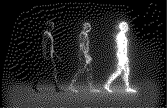
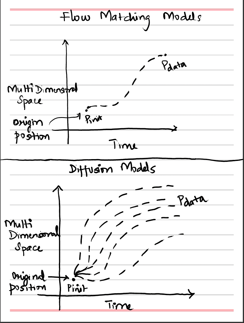
‍Diffusion models generate samples by initializing with noise (usually Gaussian noise) and iteratively applying a neural network to progressively map the noise into a sample in the training data distribution. In contrast, flow matching models parameterize a continuous-time map that directly pushes the initialized random noise toward the (training) data distribution in a single smooth trajectory (without stochasity/randomness), yielding a more direct transformation.

So far, their biggest impact has been in creative media: powering tools that can produce art, photos, and video clips. However, researchers are already exploring their use in other domains, such as text generation and molecule design, demonstrating that these models aren’t limited to visuals.

Okay, what does generating an image/video even mean?

Let’s first see how the images/videos are represented as data from the perspective of diffusion/flow-matching algorithms:

Images

An image can be represented as a three-dimensional tensor: z_image ∈ R^(H × W × 3)
where:
H = height (number of pixels vertically)
W = width (number of pixels horizontally)
3 = the color channels (RGB)
Each pixel is therefore a vector in R³, containing its red, green, and blue values.

Videos

A video is essentially a sequence (or stack) of image frames over time. It can be represented as a four-dimensional tensor:
z_video ∈ R^(T × H × W × 3)

where:
T = number of frames (temporal dimension)
H, W, and 3 are the same as in the image case

Equivalently, a video can be thought of as:
z_video = [z₁, z₂, …, z_T]
with each frame:
z_t ∈ R^(H × W × 3), t = 1, 2, …, T
Mathematically, a video is simply a sequence of stacked images indexed by time.

Let’s consider, for example, that the dataset used to train our “diffusion/flow-matching model”, which can generate images/videos, is the “entire internet”. In this context, what does it mean to generate something successfully?

Suppose the prompt is: “A picture of a dog”.

• If the model outputs pure noise, the result is useless.
• If it outputs a street photo, it’s bad (not what we asked for).
• If it generates a cat, it’s closer but still wrong.
• Only when it produces a realistic dog do we consider it successful!

These evaluations are subjective. To be more rigorous, we need to formalize criteria for what makes a generation “good.”

Formalizing quality with data distributions

One way to formalize “goodness” is by asking: How likely would this image appear on the internet for the given input prompt/query — “A picture of a dog”?

Noise → impossible
Random street photo → pretty rare
Cat → unlikely (given the prompt)
Dog → very likely

This leads us to a fundamental insight:
the quality of an image ≈ the probability of how close it is to the data in training dataset.

Generation as sampling

In theory, generation simply means picking/sampling an object from the (training) data distribution:
z ~ p_data
where:
z = the data object (e.g., an image, video, or text)

If we could sample directly from the data distribution, every output would look perfectly realistic. But here’s the problem: we don’t know the exact probability density function (PDF) of p_data.

i.e., We don’t have a closed-form distribution equation to model the
internet-scale images/videos, where we can simply sample from the distribution by using some parameters in a controlled / random way.

Example:

• Gaussian → parameters: µ (mean), σ (std)‍
• Exponential → parameter: λ (rate)‍
• Beta distribution → parameters: α and β (shape parameters)

To expand a bit more on the above, since it will provide the segway on why we need generative models:

What Is a probability density function (PDF)?

The probability density function p_data(z) tells us how likely it is to observe a data point zin the training dataset.
High value → realistic/likely
Low value → unrealistic/unlikely

It gives us a numerical measure of plausibility for every possible data object (evaluated at time t) to be present in the training dataset.

Why don’t we Know the exact PDF?

To know p_data exactly, we would need:
1. Infinite data: every possible image, video, or text sample that could exist
2. Perfect modeling: the ability to compress all of this into a single mathematical function

This is practically impossible because real-world data is too high-dimensional and complex. Even huge datasets (ImageNet, LAION, YouTube, etc.) are just approximations of the true distribution.

Why would knowing it matter?

If we somehow knew the exact p_data:

We could generate perfect samples directly
We could evaluate quality exactly (by computing probabilities)
We wouldn’t need generative models at all

But since we don’t (which would be the case when fitting to any real-world distribution), we need a model that can learn to approximate it.

This is where generative models come in

Generative models are designed to approximate the unknown data distribution.

The recipe:
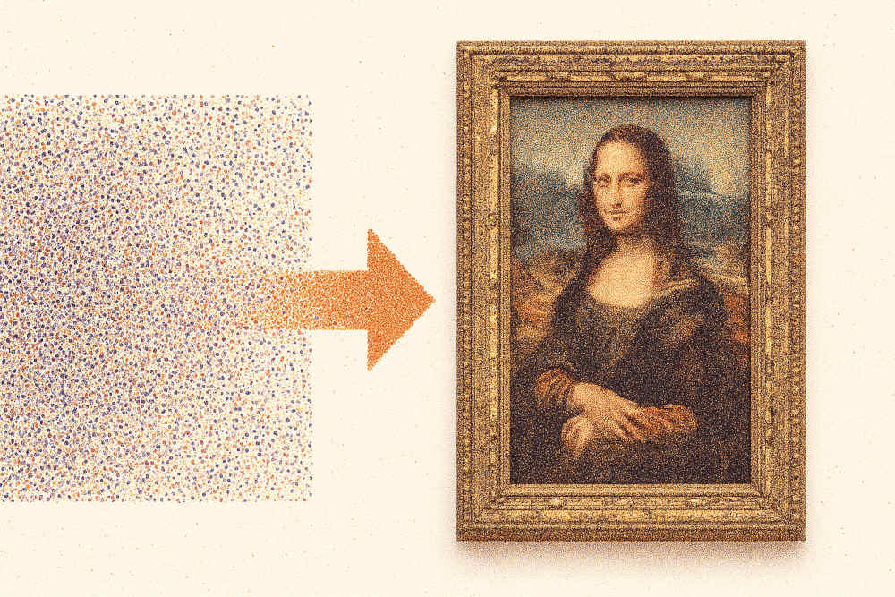
1. Start with a simple, known distribution (like Gaussian noise): x ~ N(0, I_d)
2. Train a model that transforms this simple noise into samples resembling p_data: x ~ p_init → Generative Model → z ~ p_data

This is what diffusion and flow-matching models do: they provide systematic ways to approximate p_data without ever knowing it explicitly.

Conditional generation

So far, we’ve looked at unconditional generation (just sampling any realistic object). But often we want to condition on a prompt: like “dog,” “cat,” or “white dog with black dots.”

This is modeled as a conditional distribution:
z ~ p_data(· | y)
where:
z = the output (the generated image/video)
y = the prompt or condition (text description, label, or other guiding signal)

Key distinction:
z = the data we generate
y = the instruction guiding what we generate

Now, let’s see in detail how we can accomplish the goals of approximating data distribution to produce a realistic images/videos in an unconditional/conditional-(prompted) way using Flow and Diffusion Models

Flow Models:

Imagine you have a bunch of data points (like images, text, or audio) and you want to understand how they can transform from one form to another (from random/gaussian noise to the data domain — image, text, video, etc). Flow models provide a mathematical framework to describe these transformations as smooth, continuous movements through space.

Think of it like this: instead of magically teleporting from point A to point B, flow models describe the entire journey - every step along the way.

Let’s first understand the fundamental components that constitute a flow-model:

Meaning behind Notations:
x → f(x) means "x maps to f(x)"
a : [b,c] → R^d means “Function a maps each input from interval [b,c] to a d-dimensional real vector.”
a : R^d × [b,c] → R^d means “Function a takes a d-dimensional vector and a value from interval [b,c], then outputs a d-dimensional vector.

Trajectories

A trajectory describes how a data point moves through time.
Formally, a trajectory is a function of time:

x : [0,1] → R^d
t ↦ x_t

At any given time t, the trajectory gives a vector x_t ∈ R^d.
Intuitively, you can imagine x_t as a point moving through space as time evolves.

Vector fields

A vector field tells us the direction and velocity of movement at every point in space and time.
Formally, we define:

u : R^d × [0,1] → R^d
(x,t) ↦ u_t(x)

This means: given a point x at time t, the vector field returns a direction u_t(x) showing how the trajectory should move.

6.3. Ordinary differential equation (ODE)

The trajectory x_t must be consistent with the vector field. This is expressed as an ODE:

dx_t / dt = u_t(x_t)

This says: the velocity of the trajectory (dx_t/dt) equals the vector field evaluated at the current position.

We also need an initial condition:

x_0 = x₀

which means the trajectory starts at some initial point x₀.

Flow

A flow is the collection of all trajectories that solve the ODE for different initial conditions.

Formally, we define the flow as:

Φ_t : R^d → R^d
Φ_t(x₀) = x_t

where:
Φ_t(x₀) tells us the position at time t if we started at x₀.
Each initial point x₀ generates one trajectory.
Collectively, all these trajectories form the flow.

Summary of relationships

• Vector field → defines the ODE.
• ‍ODE → determines how trajectories evolve.
• ‍Trajectory → a solution to the ODE starting at some initial condition.
• ‍Flow → the collection of trajectories for all initial conditions.

Example: Linear ODE in flow models

Let’s work through a simple but powerful example of a flow defined by a linear ODE.

The setup

We define the vector field as:

u_t(x) = -θx,   where θ > 0

This means:
If x > 0, the velocity is negative → the point moves left (toward 0).
If x < 0, the velocity is positive → the point moves right (toward 0).

No matter where we start, the vector field always points us back to the origin.

The claim

We claim that the flow is given by:

ψ_t(x₀) = exp(-θt) * x₀

Here:
x₀ is the initial condition (where the trajectory starts at t=0).
exp(-θt) is the exponential decay factor.

This formula says: as time increases, the trajectory shrinks exponentially towards the origin.

Proof

Given:

Vector field: u_t(x) = -θx where θ > 0
Proposed flow: ψ_t(x₀) = exp(-θt)x₀

Verification Process

Step 1: Check initial condition

We need to verify at t = 0 : ψ₀(x₀) = x₀

ψ₀(x₀) = exp(-θ·0)x₀ = exp(0)x₀ = 1·x₀ = x₀ ✓

Step 2: Check flow ODE

We need to verify: d/dt ψ_t(x₀) = u_t(ψ_t(x₀))

Left side (derivative of flow):
d/dt ψ_t(x₀) = d/dt[exp(-θt)x₀] = -θexp(-θt)x₀

Right side (vector field applied to flow):
u_t(ψ_t(x₀)) = u_t(exp(-θt)x₀) = -θ(exp(-θt)x₀) = -θexp(-θt)x₀

Since both sides are equal, -θexp(-θt)x₀, the flow ODE is satisfied ✓

Real-world generative modeling:

In real-world generative modeling,

The data space is high-dimensional (think: every pixel in an image frame, where each image frame is part of a stack of frames in a video).
The vector fields of the neural networks are much more complex than θx.
There’s no closed-form solution like ψ_t(x₀) = exp(-θt) * x₀.

This is why we bring in neural networks.

• Neural networks approximate the vector field u_t(x) directly.
• Once the vector field is learned, we can numerically integrate the ODE to move noise samples into realistic data samples.
• This is the foundation of flow-matching models: learn the vector field that matches the true data-generating process.

Therefore, the neural network is basically going to learn to approximate the vector-field function that tells every point in the trajectory space how to move over time to match the training data distribution.

Formalizing the flow-matching sampling mechanism in terms of pseudo-code:

Okay, we have got a taste of high-level theoretical intuition of how flow-matching models are going to predict the vector field (velocity) of data points in random noise (P_init) and guide them towards the actual data distribution (P_data) (image/video to be generated)

Now, let’s formalize this as pseudo-code to solidify our understanding a bit more

The setup

What we have:
Starting point: X₀ ~ P_init (random noise or initial data)
Goal: X₁ ~ P_data (realistic data like images)
ODE: dX_t/dt = u_t^θ(X_t) where u_t^θ is our neural network

What we need:
A way to solve this ODE numerically
The neural network u_t^θ that gives us the right velocity at each point and time

The neural network as vector field

Key insight: We parameterize the vector field u_t(x) using a neural network:
u_t^θ(x) = NeuralNetwork_θ(x, t)

What this means:
Input: Current position x and current time t
Output: Velocity vector telling us which direction to move
Parameters: θ (weights and biases) that we'll learn during training
Goal: Learn θ such that following this vector field transforms noise into realistic data

The numerical solution: Euler’s method

Since we can’t solve the ODE analytically, we use numerical integration. The simplest method is Euler’s method.

The basic idea

Instead of solving the ODE continuously, we:

1. Discretize time into small steps of size h
2. Approximate the derivative using small finite differences
3. Step forward iteratively using our neural-network to approximate this derivative

Step-by-step algorithm

Algorithm: Neural ODE Solver
Input: Initial point X₀, step size h, neural network u_θ
Output: Final point X₁

1) Set t = 0
2) Set step size h = 1/n (where n is number of steps)
3) Draw initial sample X₀ ~ P_init (e.g., random noise)
4) For i = 1, 2, ..., n-1 do:
      X_{t+h} = X_t + h × u_t^θ(X_t)
      Update t ← t + h
5) Return X₁ # (generated sample: denoised from random-noise to a sample in training data distribution - Eg: image, video, etc)

Breaking down each step

Step 1: Initialize time
t = 0
Start at the beginning of our transformation process

Step 2: Choose step size
h = 1/n
Divide the time interval [0,1] into n equal steps
Smaller h = more accurate but slower computation
Typical values: n = 100 to n = 1000

Step 3: Sample starting point
X₀ ~ P_init (Random)
For image generation: sample from Gaussian noise
For other applications: sample from the appropriate initial distribution
This becomes our “noisy” starting point

Step 4: The core iteration
X_{t+h} = X_t + h × u_t^θ(X_t)
This is the heart of Euler’s method

Step 5: Return result
Return X₁

After n steps, we've traveled from t=0 to t=1
X₁ should now be a sample from our target distribution (e.g.: a realistic image)

Mathematical intuition behind applying the Euler method X_{t+h}

From calculus, we know:
dX_t/dt ≈ (X_{t+h} - X_t)/h

From our ODE, we know:
dX_t/dt = u_t^θ(X_t)

Combining these:
(X_{t+h} - X_t)/h = u_t^θ(X_t)

Solving for X_{t+h}:
X_{t+h} = X_t + h × u_t^θ(X_t)

Physical interpretation

Think of this as a navigation system:
Current position: X_t (Where we are now)
Ask for directions: u_t^θ(X_t) (Which way should we go?)
Choose how far to travel: h (Step size)
Take the step: X_t + h × u_t^θ(X_t) (New position)

Hand-crafted simple example for mental viz

Let’s say we’re generating a 1D-latent:
Current state: X_t = [0.3, -0.7, 0.1, ...]
Neural network says: u_t^θ(X_t) = [0.1, 0.2, -0.3, ...] (how to change each pixel)
Step size: h = 0.01
Next state: X_{t+0.01} = [0.301, -0.698, 0.097, ...]

Pseudo-code: The complete picture—training vs. inference

During Training

Goal: Learn the parameters θ of our neural network

For each training batch:
  1) Sample X₀ ~ P_init
  2) Sample target X₁ ~ P_data  
  3) Use neural ODE solver to compute predicted X₁
  4) Compute loss between the predicted and actual X₁
  5) Backpropagate through the entire ODE solve
  6) Update θ

During inference (Generation)

Goal: Generate new samples

For generation:
  1) Sample X₀ ~ P_init (random noise)
  2) Use trained neural network u_θ in ODE solver
  3) Solve ODE from t=0 to t=1
  4) Return X₁ (generated sample)

Extending the above ideas to diffusion models

Now that we understand how neural ODEs work for flow models, let’s see how we can extend these ideas to diffusion models with just minor adjustments. The key insight is moving from deterministic flows to stochastic processes.

The key extension: Adding randomness iteratively at each time-step

From deterministic to STOCHASTIC

What we had (Flow Models):
Deterministic trajectories following exact paths
ODE: dX_t/dt = u_t(X_t)
Given a starting point, the path is completely determined

What we get (Diffusion Models):

Stochastic trajectories with randomness at each step
SDE: dX_t = u_t(X_t)dt + σ_t dW_t
Even with the same starting point, we get different random paths

The architecture: Neural networks for stochastic processes

The vector field component

Neural Network Structure:
u: ℝᵈ × [0,1] → ℝᵈ (x, t) ↦ u_t(x)

Breaking this down:
Input: Current position x (spatial component) + current time t (time component)
Output: Direction vector telling us how to move
Parameters: θ ∈ ℝᵏ (neural network weights that we learn)

The diffusion coefficient

Additional component:
σ: [0,1] → ℝ t ↦ σ_t

Key insights:
Maps time t to a real number
Controls how much noise to inject at each time step
The idea of diffusion coefficient: Introduce randomness/stochasticity into our ODE

Behavior patterns:
σ large → More noise, more stochasticity
σ small → Less noise, more deterministic behavior
σ = 0 → Reduces back to our original deterministic ODE

The mathematical framework: Stochastic differential equations

The complete SDE formulation

dX_t = u_t(X_t)dt + σ_t dW_t

Initial conditions:
X_0 = x_0 (Initial condition - can also be made random)
Note: “You can also make it random; let’s assume it’s fixed for now.”

Breaking down each component

Change in X_t: dX_t
Represents the infinitesimal change in our data point
This is what we’re trying to model

Drift term: u_t(X_t)dt
Change due to vector field (going in the direction of the vector field)
Deterministic component learned by the neural network
Same as our original flow models

Diffusion term: σ_t dW_t
Injecting some stochastic component/noise
This is what makes it a Brownian motion (also called Wiener process)
Adds controlled randomness to our system

Understanding Brownian Motion: The heart of stochasticity

What is Brownian Motion?

“Brownian Motion: Random walk in continuous space and random time”

Mathematical definition:
W = (W_t) where {t≥0}: A stochastic process (collection of random variables)
Stochastic process: W = (W_t) where {t≥0}, doesn’t need to stop at t=1, can go till t
Random trajectory: Each path is different, even with the same starting point

The three key properties of Brownian Motion

Property 1: Always starts at zero
W_0 = 0 (Always starts at time 0, can go till ∞)
Intuition: Every random walk starts from the origin
Practical meaning: The “baseline” for our randomness is zero

Property 2: Gaussian increments
W_t - W_s ~ N(0, (t-s)I) for 0 ≤ s ≤ t
Key insight: The difference between any two arbitrary time points follows a normal distribution/Gaussian distribution
Variance grows with time: Longer time intervals → more variance
t, s are two random/arbitrary time points

Property 3: Independent increments
W_t₁ - W_t₀, W_t₂ - W_t₁, ..., W_tₙ - W_tₙ₋₁ are all independent of each other
Time points are increasing: 0 ≤ t₀ ≤ t₁ ≤ ... ≤ tₙ (time points are increasing)
Independence: What happens in one time interval doesn’t affect another
W_t ∈ ℝᵈ (can be of arbitrary dimension d)

The continuous motion property

“Brownian Motion can be drawn without lifting a pen—which intuitively means continuous motion.”

What this means:

• Continuous paths: No sudden jumps in the process‍
• Mathematical elegance: Creates smooth, continuous transformations‍
• Visual intuition: Like drawing a continuous, wiggly line (without lifting the pen)‍
• Practical implication: No abrupt changes in our diffusion process

The Stochastic process perspective

What makes it “Stochastic”

Key insight from the diagram: Instead of one deterministic trajectory, we now have a collection of random trajectories.

Visual description of: Diffusion (SDE) vs Flow Model (ODE)

Why this extension Is powerful

1. Better modeling of real processes

• Most real-world physical processes have inherent randomness
• Image generation isn’t perfectly deterministic
• Randomness can help explore different solutions

2. Enhanced generation quality (in theory)

• Can produce multiple different outputs from the same input
• Randomness helps escape local minima (could be particularly useful if the dataset size is small)
• Leads to more diverse and realistic samples (in theory)

The flow vs. Diffusion connection

What stays the same:

• Neural networks parameterize the vector field u_t(X_t)‍
• Time evolution from t=0 to t=1
• Goal of transforming simple → complex distributions
• Numerical integration methods (with modifications — Euler vs Euler Maruyama Method [We will see this later in the doc])

Key differences—flow-matching vs diffusion models:

From theory to implementation: Making SDEs sampleable

The fundamental challenge

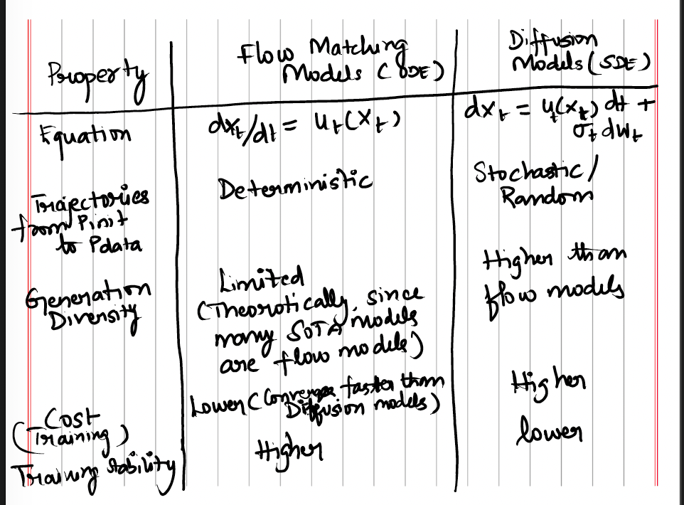
We now understand the mathematical beauty of stochastic differential equations, but there’s a crucial implementation hurdle: we can’t directly sample from a differential equation. The SDE dX_t = u_t(X_t)dt + σ_t dW_t describes continuous-time evolution, but computers work with discrete steps.

We need to transform this continuous mathematical description into a discrete algorithm that we can actually implement.

Deriving the discrete approximation

Starting from the continuous SDE: The mathematical foundation begins with our stochastic differential equation. We know that the continuous form describes the evolution of our system, but we need to find an equivalent discrete form that preserves the essential properties.

The key mathematical insight: We can derive a discrete approximation by using the fundamental definition of derivatives. From multivariable calculus, we know that:

dX_t/dt = lim(h→0) (X_{t+h} - X_t)/h = u_t(X_t)

Rearranging for practical computation: When we rearrange this equation for small but finite time steps, we get:
X_{t+h} - X_t = h × u_t(X_t) + R_h(h)
Where R_h(h) represents the error term that approaches zero as h gets smaller. This error term is a reminder that our discrete approximation becomes more accurate as we use smaller time steps. [To understand more about R_h(h), refer Extras Section 8.1 ].

The complete discrete form: For the stochastic case, we get the equivalent discrete form:
X_{t+h} = X_t + h × u_t(X_t) + h × R_t(h)

This form now doesn’t rely on derivatives and can be directly implemented in code.

Adding the Stochastic component

Incorporating Brownian motion: We’ve handled the deterministic part, but now we need to add the stochastic term σ_t dW_t. From our understanding of Brownian motion, we know that:
W_{t+h} - W_t ~ N(0, h×I_d)

This tells us that the difference in Brownian motion over a small time interval follows a normal distribution with variance proportional to the time step.

The complete stochastic update:
Combining everything, we get:
X_{t+h} = X_t + h × u_t(X_t) + σ_t(W_{t+h} - W_t) + h × R_t(h)

Simplifying for implementation: Since W_{t+h} - W_t ~ N(0, h×I_d), we can sample this difference directly:
X_{t+h} = X_t + h × u_t(X_t) + σ_t × √h × ε
Where ε ~ N(0, I_d) is a standard normal random variable.

Why the √h scaling?

Understanding the √h scaling factor is crucial for the proper implementation of stochastic differential equations. This scaling comes directly from the mathematical properties of Brownian motion.

Property of Brownian Motion
The increment of Brownian motion over an interval of length h is distributed as:
W_{t+h} - W_t ~ N(0, h)

This means the increment has:
Mean: 0 (no systematic bias)
Variance: h (grows linearly with time interval)

The key implication

Since variance measures the square of the “typical size” of fluctuations, the standard deviation (the actual scale of random jumps) is:
Standard deviation = √(variance) = √h

Important insight: Randomness in Brownian motion grows with the square root of elapsed time, not linearly with time. This is a fundamental property that distinguishes Brownian motion from simple linear processes.

How we simulate it in practice

To generate the correct increment in discrete time steps:

1. Start with a standard Gaussian: Sample ε ~ N(0,1)
2. Scale appropriately: Multiply by √h
   ΔW ≈ √h × ε

Why this scaling works:
This scaling ensures the variance matches the theoretical requirement:
Var(√h × ε) = h × Var(ε) = h × 1 = h ✓

The mathematical verification:
We need: Var(W_{t+h} — W_t) = h
We know: W_{t+h} — W_t = √h × ε
Therefore, Var(√h × ε) = h × Var(ε) = h × 1 = h
The scaling preserves the correct statistical properties

In code, this translates to:
epsilon = torch.randn_like(x) # Sample from N(0,1)
brownian_increment = math.sqrt(h) * epsilon

This √h scaling is essential for maintaining the mathematical integrity of the stochastic process during numerical simulation.

The complete diffusion model sampling algorithm

Algorithm: Sampling from SDE (Euler Maruyama Method)

Input: 
- Vector field u_t (neural network)
- Number of steps n
- Diffusion coefficient σ_t

1) Set t = 0
2) Step size h = 1/n  
3) X_0 = x_0 (starting condition - random noise)
4) For i = 1, ..., n-1 do:
      # Draw a sample from a standard Gaussian  
      ε ~ N(0, I_d)  # because the time steps differ by h
      
      # Add additional noise with variance h 
      # scaled by diffusion coefficient σ_t
      X_{t+h} = X_t + h × u_t(X_t) + σ_t × √h × ε
      
      Update t ← t + h
5) Return X_0, X_h, X_{2h}, X_{3h}, ..., X_1 
# (X1 is approximately a sample in the training data distribution)

Key implementation details:

Step size considerations: The step size h = 1/n determines both accuracy and computational cost. Smaller h gives more accurate results but requires more computation.

Noise sampling: At each step, we sample ε from a standard normal distribution N(0, I_d). This is computationally efficient and maintains the independence property of Brownian motion increments.

Scaling by diffusion coefficient: The term σ_t × √h × ε properly scales the noise according to our diffusion schedule and the time step size.

Extras [skippable section]

Understanding the Error Term R_h(h)

The error term R_h(h) represents the difference between our discrete approximation and the true continuous solution. Let’s explore this with a concrete example.

Simple Example: Linear Growth
Consider the simple ODE:
dx/dt = 2x
x(0) = 1

The exact solution is: x(t) = e^(2t)

Our discrete approximation using Euler’s method:
x_{t+h} = x_t + h × (2x_t) = x_t(1 + 2h)

Comparing Exact vs. Approximate
Let’s see what happens at t = 0.1 with step size h = 0.1:

Exact solution:
x(0.1) = e^(2×0.1) = e^0.2 ≈ 1.2214

Discrete approximation:
x_{0.1} = x_0 × (1 + 2×0.1) = 1 × (1.2) = 1.2000

The error term:
R_h(h) = True value - Approximation = 1.2214 - 1.2000 = 0.0214

How Error Decreases with Smaller Steps
Let’s try with h = 0.05 (two steps of 0.05 each):

Step 1: x_{0.05} = 1 × (1 + 2×0.05) = 1.1
Step 2: x_{0.1} = 1.1 × (1 + 2×0.05) = 1.1 × 1.1 = 1.21
New error: R_h(h) = 1.2214 - 1.21 = 0.0114

Conclusion for

We began with a simple question: What does it mean to generate something realistically? Along the way, we saw how images and videos can be mathematically represented, how their quality can be formalized using probability distributions, and why the exact probability density function of real-world data is impossible to know.

This challenge is exactly where generative models step in. By starting from simple, well-understood distributions (like Gaussian noise) and learning to transform them into complex data distributions, these models allow us to approximate the true p_data.

• Flow models give us a deterministic framework: transforming noise into data by following continuous vector fields described by ODEs.
• Diffusion models extend this by adding stochasticity: injecting randomness through SDEs, which often leads to richer and more diverse generations.
• In both cases, the missing piece, the unknown vector field, is learned by a neural network, which acts as the guide that tells noisy samples how to gradually evolve into realistic data.

From a practical perspective, this has given rise to tools that can generate artwork, videos, text, molecules, and beyond, reshaping how humans create and interact with information. Some examples of the video-generation models where Diffusion/Flow-Matching models form the core backbone are:
Tavus’ Phoenix-3, Google’s Veo-3, Meta’s MovieGen, etc.

Note: This is a summary of an article written on our researcher, Karthik's Medium. Follow him for the latest.

Ready to converse?

Get started with a free Tavus account and begin exploring the endless possibilities of CVI.

GET STARTED