
All Posts
Research
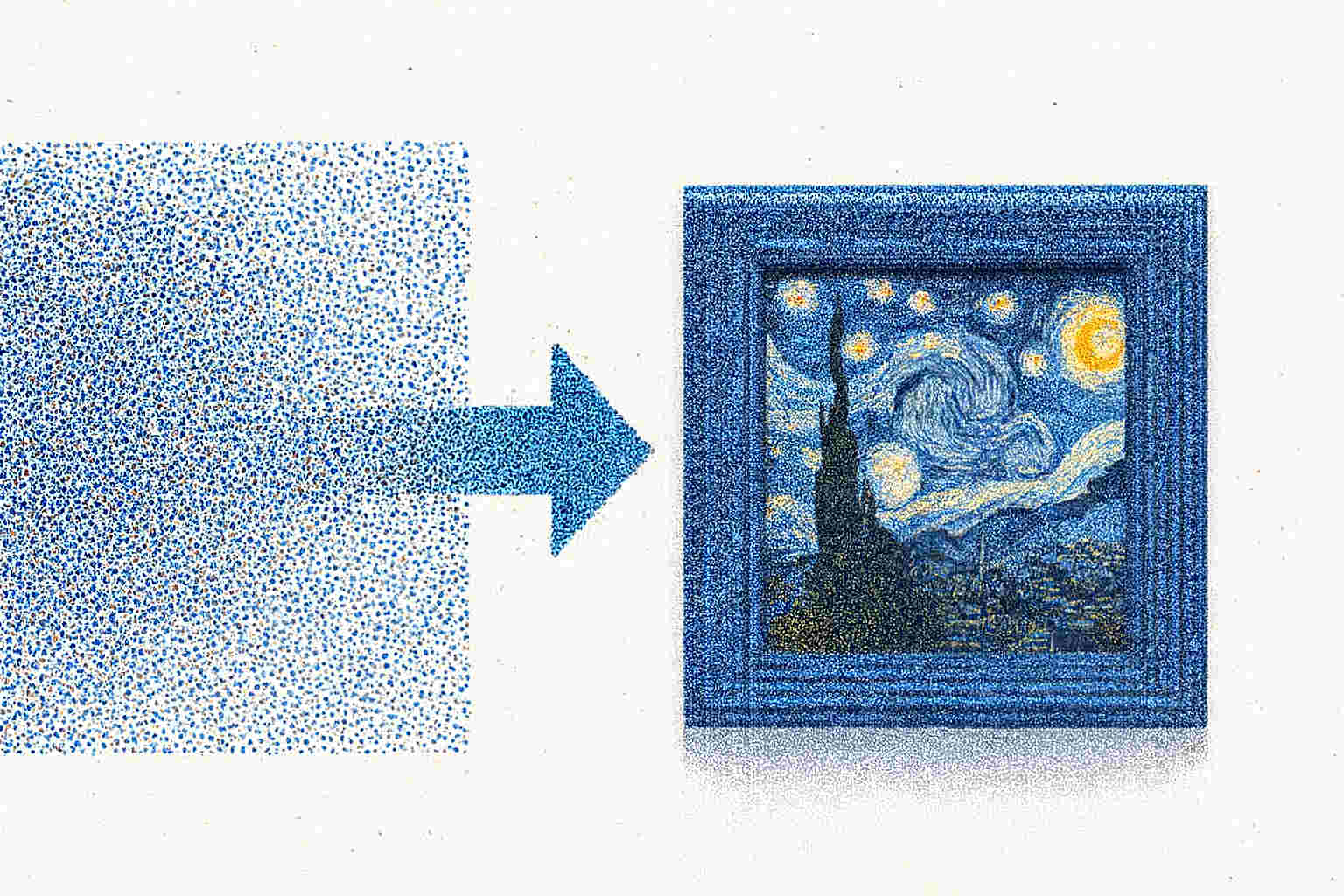
From random noise to real images: Understanding loss-function formulation
Written by

Karthik Ragunath Ananda Kumar
All Posts
Written by
Karthik Ragunath Ananda Kumar
In Part 1, we established the mathematical foundations of flow matching and diffusion models—from deterministic ODEs (dX_t/dt = u_t(X_t)) to stochastic SDEs (dX_t = u_t(X_t)dt + σ_t dW_t) and their numerical implementation.
The crucial question remained: How do we actually train these models?
This part focuses on understanding the intuition behind constructing training targets (or) loss functions from a code implementation POV to train diffusion/flow-matching neural nets.
We’ll cover probability path construction, conditional vs. marginal formulations, and practical training target design.
Any probability path that can be used for training must satisfy two critical mathematical conditions:
Condition 1: Probability Distribution Property
P_t(·|z) must be a valid probability distribution for all t ∈ [0,1]Condition 2: Boundary Conditions
P_0(·|z) ≈ P_init (starts from noise, independent of target z)P_1(·|z) = δ_z (ends at exact data point z with zero variance)Why are these conditions essential?
As noted in the mathematical literature, “the distribution collapses stepwise into a single data point” - this captures the essence of how we transform broad uncertainty (noise) into perfect certainty (exact target).
The most widely used probability path is the Gaussian construction:
P_t(·|z) = N(α_t z, β_t² I_d)
Breaking down each component:
P_t(·|z): Probability distribution at time t, conditioned on target zN(μ, σ²): Gaussian distribution with mean μ and variance σ²α_t z: Time-dependent means that it gradually moves toward the target zβ_t² I_d: Time-dependent variance that shrinks to zeroz: Target data point (could be an image, text, etc.)Boundary requirements:
α_0 = 0, α_1 = 1 (mean interpolates from 0 to target)β_0 = 1, β_1 = 0 (variance interpolates from maximum to zero)Linear scheduling example:
α_t = t (signal strength grows linearly) β_t = 1 - t (noise level decreases linearly)
Condition 1 verification:
∫ N(α_t z, β_t² I_d) dx = 1Condition 2 verification:
t = 0: P_0(·|z) = N(0·z, 1²·I) = N(0, I) = P_init ✓
t = 1: P_1(·|z) = N(1·z, 0²·I) = δ_z ✓
The Dirac Distribution Insight: At t = 1, we get δ_z (Dirac distribution) - a mathematical object representing perfect certainty. Think of it as something like a GPS coordinate with zero error: while normal distributions say “you’re somewhere in this neighborhood,” the Dirac distribution says “you’re at exactly this address.”
The marginal distribution emerges from combining all conditional paths:
P_t(x) = ∫ P_t(x|z) P_data(z) dz
What each component means:
P_t(x|z): “Given target z, what’s the probability of being at x at time t?”P_data(z): “How likely is z to appear in our training data?”P_t(x): “Overall, what’s the probability of being at x at time t?”Intuitive interpretation: We’re taking a weighted average of all conditional paths, where weights are determined by how common each data point is in our training set.
Scenario: Training on a dataset with three images: cat (z₁), dog (z₂), bird (z₃), each equally likely.
Individual conditional paths:
P_t(·|cat) = N(α_t × cat_image, β_t² I): Path from noise to catP_t(·|dog) = N(α_t × dog_image, β_t² I): Path from noise to dogP_t(·|bird) = N(α_t × bird_image, β_t² I): Path from noise to birdMarginal combination:
P_t(x) = (1/3)[P_t(x|cat) + P_t(x|dog) + P_t(x|bird)]
At t = 0 (start):
N(0, I) (same Gaussian noise)P_0(x) = N(0, I) (single Gaussian)At t = 0.5 (middle):
N(0.5×z_i, 0.25I) for each target z_iAt t = 1 (end):
δ_cat, δ_dog, δ_bird (exact points)The marginal automatically satisfies our conditions:
Let’s carefully derive why the marginal distribution inherits the required properties from the conditional distributions.
Mathematical proof: Since each conditional path P_t(x|z) is a valid probability distribution:
∫ P_t(x|z) dx = 1 for all z
And since P_data(z) is a valid probability distribution over training data:
∫ P_data(z) dz = 1
The marginal distribution:
P_t(x) = ∫ P_t(x|z) P_data(z) dz
Verification that it integrates to 1:
∫ P_t(x) dx = ∫ [∫ P_t(x|z) P_data(z) dz] dx
= ∫ P_data(z) [∫ P_t(x|z) dx] dz (swap integration order)
= ∫ P_data(z) × 1 dz (since ∫ P_t(x|z) dx = 1)
= ∫ P_data(z) dz = 1 (since P_data is valid)
Intuition: A weighted average of probability distributions is also a probability distribution.
At t = 0:
Starting from our Gaussian conditional paths:
P_0(x|z) = N(α_0 z, β_0² I)
= N(0·z, 1²·I)
= N(0, I)
Notice that at t = 0, the conditional distribution doesn’t depend on z anymore!
Marginal at t = 0:
P_0(x) = ∫ P_0(x|z) P_data(z) dz
= ∫ N(0, I) P_data(z) dz
= N(0, I) ∫ P_data(z) dz (N(0,I) doesn’t depend on z)
= N(0, I) × 1 (since P_data integrates to 1)
= N(0, I)
At t = 1:
Starting from our conditional paths:
P_1(x|z) = N(α_1 z, β_1² I)
= N(1·z, 0²·I)
= δ_z
Marginal at t = 1:
P_1(x) = ∫ P_1(x|z) P_data(z) dz
= ∫ δ_z P_data(z) dz
Using the fundamental property of Dirac distributions: For any function f(z): ∫ f(z) δ_z(x) dz = f(x) (the Dirac “picks out” the value at x)
Therefore:
P_1(x) = ∫ δ_z P_data(z) dz
= P_data(x)
Let’s verify this with our cat, dog, and bird example, where each has a probability of 1/3.
Training data distribution:
P_data(z) = { 1/3 if z = cat_image 1/3 if z = dog_image 1/3 if z = bird_image 0 otherwise }
At t = 0 verification:
P_0(x) = (1/3)P_0(x|cat) + (1/3)P_0(x|dog) + (1/3)P_0(x|bird)
= (1/3)N(0,I) + (1/3)N(0,I) + (1/3)N(0,I)
= N(0,I)
All conditional paths at t=0 are identical, so their weighted average is the same distribution.
At t = 1 verification:
P_1(x) = (1/3)P_1(x|cat) + (1/3)P_1(x|dog) + (1/3)P_1(x|bird)
= (1/3)δ_cat + (1/3)δ_dog + (1/3)δ_bird
This gives us a distribution that puts probability mass 1/3 at each training image location, which exactly matches our training data distribution P_data(x).
Individual correctness → Collective correctness:
Practical implication: When we train on individual conditional paths P_t(x|z), we’re automatically learning the correct marginal behavior P_t(x) without ever computing it explicitly.
Training perspective:
# During training
for each_step:
    z = sample_from_training_data()
    # Gets cat, dog, or bird with prob 1/3 each

    x = sample_from_conditional_path(z, t)
    # Sample from P_t(x|z)

    # Train network on this (x, z) pair
    # Result after training:
    # Network learned to handle all conditional paths# Automatically produces correct marginal behavior
This mathematical framework ensures that by solving many individual problems correctly, we automatically solve the collective problem correctly.
Now that we have established how probability paths P_t(·|z) provide the mathematical foundation for transforming noise into data. We showed how individual conditional paths combine to create meaningful marginal distributions that satisfy our boundary conditions.
Now comes the crucial question: How do neural networks actually learn to follow these paths?
The answer lies in vector fields - the mathematical objects that neural networks learn to approximate. While probability paths tell us where points should be at each time, vector fields tell us how to get there by specifying the direction and speed of movement at every location.
This part bridges the gap between mathematical theory and practical implementation, showing how:
Vector fields are fundamental to understanding how probability distributions evolve over time. In machine learning, particularly in diffusion models and flow matching, we need to understand two key concepts: conditional vector fields and marginal vector fields.
Before diving into conditional and marginal concepts, let’s understand what a vector field is.
Intuition: Imagine you’re watching particles floating in water. At each point in space, the water current pushes the particle in a particular direction with a particular speed. A vector field is simply a function that tells you, at any point in space and time, which direction and how fast things should move.
Mathematically, if we have a point x at time t, a vector field u_t(x) tells us the velocity at that location:
dx/dt = u_t(x)
This equation says: “the rate of change of position equals the velocity given by the vector field.”
In generative modeling, we want to train a neural network to learn a vector field that transforms simple noise (like a Gaussian distribution) into complex data (like images). But what exactly should we train the network to predict?
The answer lies in understanding conditional and marginal vector fields.
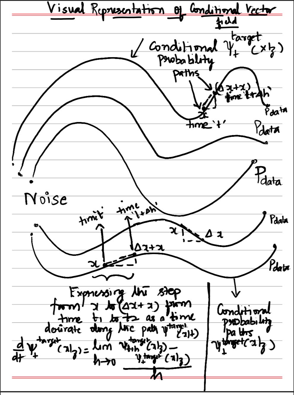
Conditional means “given specific information.” A conditional vector field u^target_t(x|z) tells us: “What velocity should we have at position x and time t, given that we’re trying to reach a specific target data point z?”
For each data point z, we define a probability path p_t(·|z) that describes how noise gradually becomes z. A common choice is gaussian probability path which is given by:
p_t(x|z) = N(α_t z, β_t² I)
Let’s understand what this means and why we use this specific form.
A probability path p_t(x|z) is a time-indexed family of probability distributions that describes how a random variable evolves from time t=0 to t=1.
Think of it as a movie showing how a cloud of particles transforms over time:
The mean: α_t z
The mean of the distribution moves from 0 (at t=0) to z (at t=1). The scheduler α_t controls this interpolation:
The variance: β_t² I
The variance controls how “spread out” the distribution is. The scheduler β_t controls how noisy the samples are:
The I is the identity matrix, meaning the variance is the same in all directions (isotropic).
Let’s say z = [5, 5] (a point in 2D space) and use simple schedulers:
At t = 0:
p_0(x|z) = N(0·[5,5], 1² I) = N([0,0], I)
This is a standard Gaussian centered at the origin. If you sample from it, you might get points like:
These are scattered randomly around [0, 0] with no knowledge of where z is.
At t = 0.5:
p_0.5(x|z) = N(0.5·[5,5], 0.5² I) = N([2.5, 2.5], 0.25 I)
Now the cloud has moved! It’s centered at [2.5, 2.5] (halfway to the target) and is less spread out (variance reduced to 0.25). Sample points might be:
Notice they’re closer to each other and closer to the target.
At t = 0.9:
p_0.9(x|z) = N(0.9·[5,5], 0.1² I) = N([4.5, 4.5], 0.01 I)
Now the cloud is very concentrated near [4.5, 4.5], very close to the target [5, 5]. Sample points might be:
They’re all very close to the target with very little noise.
At t = 1:
p_1(x|z) = N(1·[5,5], 0² I) = δ([5,5])
This is a Dirac delta function - all samples are exactly at [5, 5]. No randomness left.
There are several deep reasons why this specific form is so powerful:
1. Smoothly Interpolates Between Noise and Data
We need a path that:
The Gaussian form with time-varying mean and variance achieves this smoothly. There are no discontinuities or jumps - the transformation is gradual and continuous.
2. Mathematically Tractable
Gaussians have beautiful properties:
This makes both training and inference computationally feasible. With other distributions, we’d need expensive numerical integration or approximations.
3. Separates Signal and Noise Cleanly
The form α_t z + β_t x_0 (where x_0 ~ N(0,I)) beautifully separates:
This separation makes it clear what the model needs to learn: given a noisy observation, predict the clean signal. This is exactly the denoising problem that neural networks excel at.
4. Flexible via Schedulers
Different choices of α_t and β_t give different behaviors:
Linear schedulers (α_t = t, β_t = 1-t):
Cosine schedulers:
Variance-preserving (α_t² + β_t² = 1):
5. Alternative Perspective: Weighted Interpolation
You can also think of this as a weighted interpolation:
x_t ~ p_t(x|z) means x_t = α_t z + β_t ε, where ε ~ N(0, I)
At any time t, each sample is a weighted combination of:
As time progresses:
This is intuitive: we gradually add more “data-ness” and remove “noise-ness”.
Why not uniform distributions?
Why not mixture models?
Why not exponential or other distributions?
The schedulers α_t and β_t control this transition and must satisfy certain properties:
At t=0 (pure noise):
At t=1 (pure data):
Properties we want:
Now that we understand the probability path, we can derive the vector field that achieves it:
u^target_t(x|z) = (α’_t - (β’_t/β_t)α_t)z + (β’_t/β_t)x
Where α’_t and β’_t are time derivatives (rates of change) of the schedulers.
Let’s understand each component:
(α’_t - (β’_t/β_t)α_t)z(β’_t/β_t)x(β’_t/β_t) is the relative rate of change of noiseLet’s derive why this formula works.
Step 1: Define the flow
We construct a deterministic mapping from noise to data:
ψ^target_t(x|z) = α_t z + β_t x
This says: “Take noise x, scale it by β_t, and add α_t times the target z.”
Intuition: This is a simple linear interpolation. When we apply this transformation to standard Gaussian noise, it produces the probability distribution we want.
Step 2: Verify the distribution
If X_0 ~ N(0, I) (standard Gaussian noise), then:
X_t = ψ^target_t(X_0|z) = α_t z + β_t X_0
Since X_0 is Gaussian with mean 0 and variance I, and we’re applying a linear transformation, X_t is also Gaussian with:
This matches our desired probability path p_t(·|z) = N(α_t z, β_t² I). ✓
Step 3: Extract the vector field
The vector field is the time derivative of the flow. By the definition of a flow:
d/dt ψ^target_t(x|z) = u^target_t(ψ^target_t(x|z)|z)
The above equation says: “The rate of change of the flow equals the vector field evaluated at the current position”. In simpler words, this means, with the trained (target) conditional vector-field model, which can evaluate/approximate the vector fields at each point along the conditional probability distribution path, if we take sequential differential steps in the direction given by the vector field at each point, starting from random noise, it’s equivalent to following the conditional probability path from noise to data distribution.
Taking the time derivative of the left side:
d/dt(α_t z + β_t x) = α’_t z + β’_t x
For the right side, we need u^target_t evaluated at ψ^target_t(x|z) = α_t z + β_t x.
Setting them equal:
α’_t z + β’_t x = u^target_t(α_t z + β_t x|z)
Step 4: Change variables
The equation above tells us the vector field value at the specific point (α_t z + β_t x). But we want a formula that works for any arbitrary point in space.
The insight: As x ranges over all possible values in ℝ^d, the expression (α_t z + β_t x) also ranges over all possible points in ℝ^d. We’re just scaling and shifting, which still covers all of space.
The substitution: Let’s rename (α_t z + β_t x) as x’ to represent “any arbitrary point where we want to evaluate the vector field.”
So we define: x’ = α_t z + β_t x
Solving for x in terms of x’:
x = (x’ - α_t z)/β_t
Now substitute this back into our equation. The left side becomes:
α’_t z + β’_t x = α’_t z + β’_t · [(x’ - α_t z)/β_t]
= α’_t z + (β’_t/β_t)(x’ - α_t z)
And our equation becomes:
α’_t z + (β’_t/β_t)(x’ - α_t z) = u^target_t(x’|z)
Why this works: We’re essentially saying, “for the equation to hold for all possible values of x, it must hold for all possible points in space. So let’s just call an arbitrary point x’ and express everything in terms of that.”
Analogy: Suppose you know that f(2y + 3) = y² + 1 for all y. You want a formula for f(w) for any w.
w = 2y + 3y = (w - 3)/2f(w) = [(w-3)/2]² + 1Same principle - we’re expressing the function in terms of its actual input variable rather than an intermediate variable.
Step 5: Simplify
α’_t z + (β’_t/β_t)x’ - (β’_t/β_t)α_t z = u^target_t(x’|z)
Collecting terms with z and x’:
α’_t z - (β’_t/β_t)α_t z + (β’_t/β_t)x’ = u^target_t(x’|z) [α’_t - (β’_t/β_t)α_t]z + (β’_t/β_t)x’ = u^target_t(x’|z)
Dropping the prime notation (since this holds for any point, we can just call it x):
u^target_t(x|z) = [α’_t - (β’_t/β_t)α_t]z + (β’_t/β_t)x
This is exactly our conditional Gaussian vector field! ✓
Think of this vector field as having two competing forces:
As time progresses:
Now that we understand conditional vector fields thoroughly. Let’s see how they combine to form the marginal vector field.
While the conditional vector field u_t(x|z) handles a single data point z, in practice we have many data points from a distribution p_data(z). The marginal vector field is the average behavior across all possible targets.
Intuition: Imagine you’re at a noisy location x at time t. You don’t know which specific data point you’re heading toward. The marginal vector field tells you the best direction to move on average, considering all possible destinations weighted by their likelihood.
u^target_t(x) = ∫ u^target_t(x|z) p_t(z|x) p_data(z) dz / p_t(x)
Let’s break this down:
This integral says: “Average the conditional vector field over all data points z, weighted by how likely each z is given our current position x.”
This can be proven by using the continuity-equation.
Let’s start with the equation that governs how probability flows through space:
∂p_t(x)/∂t = -∇·(p_t(x) u_t(x))(Equation 1)
This is our continuity equation. It’s saying something profound but simple: probability doesn’t magically appear or vanish - it just flows from one place to another.
Let me break down what each piece means:
p_t(x) - This is the probability density at position x and time t. Think of it as “how much stuff is at this location right now?”
u_t(x) - This is the velocity field, and it’s really the star of the show. At every point x in space, this tells you “which direction should things move, and how fast?”
For example, if u_t(x) = z - x, it means “flow toward a point z.” Particles literally follow this field - their positions evolve according to dx_t/dt = u_t(x_t).
p_t(x) u_t(x) - This product is the probability flux. It captures both where things are going (direction from u_t) and how much is going there (scaled by density p_t). Dense regions moving fast create large flux; sparse regions moving slowly create small flux.
∇·(p_t u_t) - The divergence measures whether flow is spreading out or converging:
The negative sign - This is what makes the physics work. If divergence is positive (stuff leaving), we need density to decrease, hence the negative sign. If divergence is negative (stuff arriving), density increases, which the negative sign handles correctly.
So equation (1) is really just saying: the rate at which density changes at a point equals how much flow is leaving or entering that point.
Here’s the scenario in generative modeling. We don’t have just one target to flow toward - we have an entire dataset of targets.
We have several probability distributions to keep track of:
Data distribution p_data(z)
p_data(z)(Equation 2)
This is your training data - could be thousands of images, each one a potential target z.
Conditional probability path p_t(x|z)This answers: “If I’m trying to generate a specific image z, What’s the probability I’m at position x at time t?” Each target has its own probability path.
Conditional vector field u^target_t(x|z)For each target z, there’s a velocity field that tells you how to flow toward it. And importantly, each of these satisfies its own continuity equation:
∂p_t(x|z)/∂t = -∇·(p_t(x|z) u^target_t(x|z))(Equation 3)
Notice how this is just equation (1), but for each specific conditional distribution.
Marginal distribution p_t(x)
Now here’s where things get interesting. The overall probability at position x needs to account for all possible targets:p_t(x) = ∫ p_t(x|z) p_data(z) dz(Equation 4)
We’re summing up (integrating over) the conditional probabilities weighted by how likely each target is in the training data.
The question: What’s the velocity field u^target_t(x) for this marginal distribution? In other words, when you could be flowing toward any target in the dataset, what’s your effective velocity?
Starting with equation (4), let’s take the time derivative:∂p_t(x)/∂t = ∫ ∂p_t(x|z)/∂t p_data(z) dz(Equation 5)
I just moved the time derivative inside the integral. The p_data(z) doesn’t change with time, so it comes along for the ride.
What this says: the total density changes as each conditional density changes.
From equation (3), we know how each p_t(x|z) evolves:∂p_t(x|z)/∂t = -∇·(p_t(x|z) u^target_t(x|z))
Let me plug this into equation (5):∂p_t(x)/∂t = ∫ [-∇·(p_t(x|z) u^target_t(x|z))] p_data(z) dz(Equation 6)
The intuition here is straightforward: each target creates its own “river” with velocity u^target_t(x|z), and we’re summing up how all these rivers change the total density.
The divergence operator ∇ works on the variable x, while our integral is over z. These are independent variables, so we can swap their order:
∂p_t(x)/∂t = -∇·(∫ p_t(x|z) u^target_t(x|z) p_data(z) dz)(Equation 7)
Think of it this way: the divergence of a sum equals the sum of divergences. We’re combining all the individual probability fluxes into one total flux.
Now, we want the marginal distribution to follow its own continuity equation. There should exist an effective velocity field u^target_t(x) such that:∂p_t(x)/∂t = -∇·(p_t(x) u^target_t(x))(Equation 8)
This is just equation (1), but for the marginal distribution. We’re demanding that total probability also flows smoothly.
Look at equations (7) and (8). Both equal ∂p_t(x)/∂t, so the right-hand sides must be equal:
∇·(p_t(x) u^target_t(x)) = -∇·(∫ p_t(x|z) u^target_t(x|z) p_data(z) dz)Cancel the negative signs and divergences:
p_t(x) u^target_t(x) = ∫ p_t(x|z) u^target_t(x|z) p_data(z) dz(Equation 9)
This is saying: the total probability flux equals the sum of all conditional fluxes.
From equation (9), divide both sides by p_t(x):
u^target_t(x) = ∫ u^target_t(x|z) p_t(x|z) p_data(z) dz / p_t(x)(Equation 10)
The marginal velocity is a weighted average of the conditional velocities.
Equation 10 is exactly equal to the ‘Marginal Vector Field Formula” which we had put out earlier. Thus, we proved it.
Here’s where Bayes’ theorem comes in handy.
We know:p_t(z|x) = p_t(x|z) p_data(z) / p_t(x) (Equation 11)
This is the posterior - given you’re at position x, what’s the probability you’re heading toward the target z?
Using equation (11), I can rewrite the numerator in equation (10):p_t(x|z) p_data(z) = p_t(z|x) p_t(x)
Substituting this into equation (10):u^target_t(x) = ∫ u^target_t(x|z) p_t(z|x) p_t(x) dz / p_t(x)
The p_t(x) terms cancel:u^target_t(x) = ∫ u^target_t(x|z) p_t(z|x) dz(Equation 12)
Equation (12) is telling us something beautiful:
u^target_t(x) = ∫ u^target_t(x|z) p_t(z|x) dz
The marginal velocity at position x is the average of all the conditional velocities, weighted by the posterior probability.
Let me put this in plain language. Imagine you’re standing at position x, and you need to decide which way to move. But here’s the catch - you’re not entirely sure which target z you’re supposed to be flowing toward.
z gives you advice: u^target_t(x|z) says “hey, if you’re coming to me, go this direction”p_t(z|x) - the probability that you’re actually heading toward that targetLet’s say you’re generating images and you’re at some partially denoised position x.
Early on (t ≈ 0): Everything’s super noisy
x could plausibly become a cat image or a dog imagep_t(z_cat|x) ≈ 0.5 and p_t(z_dog|x) ≈ 0.5Halfway there (t ≈ 0.5): Things are getting clearer
x is starting to look more cat-likep_t(z_cat|x) ≈ 0.8 and p_t(z_dog|x) ≈ 0.2Almost done (t ≈ 0.9): It’s pretty much decided
x clearly looks like one specific cat from the training setp_t(z_that_specific_cat|x) ≈ 0.95Thus, we derived it from one fundamental requirement: probability density must be conserved (continuity equation).
In the previous section, we derived that the marginal vector field should be:
u^target_t(x) = ∫ u^target_t(x|z) p_t(z|x) dz(Equation 1, from previous derivation)
This is beautiful mathematically, but there’s a problem: we can’t actually use this for training. Let me show you why, and more importantly, how flow matching elegantly solves this problem.
Here’s what we’re trying to do:
Goal: Train a neural network u_t^θ(x) to approximate the marginal vector field u_t^target(x)
If we succeed, then we can:
x_0 ~ N(0, I)dx_t/dt = u_t^θ(x_t)x_1 ~ p_dataThe question is: how do we train this network?
The most obvious thing to try is a mean-squared error loss:
L_fm(θ) = E[||u_t^θ(x) - u_t^target(x)||^2](Equation 2)
Where the expectation is over:
t ~ Uniform[0, 1]z ~ p_data (sample from dataloader)x ~ p_t(·|z) (draw from the conditional probability path at time t)What this loss says:
“Pick a random time t, pick a random data point z from your dataset, sample a noisy position x that you’d get at the time t when flowing toward z, then check how well your network’s prediction matches the true target velocity.”
Why this makes sense:
u_t^θ(x) = u_t^target(x) everywhere, the loss is 0 (perfect!)Here’s the catch. Look at equation (2) - it requires computing u_t^target(x). But from equation (1), we know:
u_t^target(x) = ∫ u^target_t(x|z) p_t(z|x) dz
And from our earlier derivation, this can be written as:
u_t^target(x) = ∫ u^target_t(x|z) p_t(x|z) p_data(z) dz / p_t(x)(Equation 3)
Why is this intractable?
To evaluate equation (3), we’d need to:
zp_t(x|z) for each onep_t(x) = ∫ p_t(x|z) p_data(z) dz - another integral over the whole dataset!Computational cost: O(N) per training example, where N = dataset size (millions of images!)
This is completely impractical. We’re stuck in a circular dependency:
u_t^target(x) to train our modelu_t^target(x) requires evaluating it against the entire datasetSimple analogy: It’s like trying to learn the average height of people in a city by measuring everyone in the city before taking each single training step. Impossible!
Instead of trying to match the intractable marginal flow u_t^target(x), what if we train on the conditional flows u^target_t(x|z) directly?
Define the Conditional Flow Matching Loss:
L_cfm(θ) = E[||u_t^θ(x) - u^target_t(x|z)||^2](Equation 4)
Where:
t ~ Uniform[0, 1]z ~ p_data (sample one data point from dataloader)x ~ p_t(·|z) (conditional probability path)Remember, for a Gaussian conditional path:
p_t(x|z) = N(α_t z, β_t^2 I)
The conditional vector field has a closed-form analytical formula:
u^target_t(x|z) = (α’_t - (β’_t/β_t)α_t)z + (β’_t/β_t)x (Equation 5)
What makes this tractable:
α_t and β_t - We chose them! (e.g., α_t = t, β_t = 1-t)α’_t and β’_tExample: For the simplest case where α_t = t and β_t = 1-t:
α’_t = 1 and β’_t = -1u^target_t(x|z) = (z - x)/(1-t)Here’s the concern: The conditional vector field u^target_t(x|z) optimizes for flowing toward a single data point z, but we want to flow toward the entire distribution p_data.
Training on conditionals seems like the wrong thing to do!
The magic: These two losses are equivalent (up to a constant)!
There exists a constant C (independent of θ) such that:
L_fm(θ) = L_cfm(θ) + C(Equation 6)
What this means:
If you plot both loss functions as a function of the parameter θ:
θ*∇_θ L_fm(θ) = ∇_θ L_cfm(θ)Why gradients being equal matters:
When we train with gradient descent, we only care about gradients:
∇_θ(L_fm(θ)) = ∇_θ(L_cfm(θ) + C) = ∇_θ L_cfm(θ)
Since C is constant, its gradient is zero!
Therefore, Stochastic gradient descent on L_cfm is exactly the same as on L_fm.
Think about what happens when we minimize the conditional flow matching loss over the entire dataset:
During training:
z ~ p_dataz, we sample noisy positions x ~ p_t(x|z)u^target_t(x|z) for each pairWhat the network learns:
x that are clearly heading toward cats, it sees many cat examples during trainingx that could be heading toward cats OR dogs; it sees examples of bothp_t(z|x)!Connection to marginal flow:
Remember the continuity equation for the marginal:
d/dt p_t(x) = -div(p_t v_t)(x)
where div measures the inflow-outflow of probability mass as we follow the conditional probability paths v_t.
By training on conditional flows sampled from the data distribution, the network learns the divergence structure that conserves the marginal probability!
Let’s get concrete. For the Gaussian conditional path:
p_t(·|z) = N(α_t z, β_t^2 I_d)
(Equation 7)
Common choice (Optimal Transport path):
α_0 = 0, α_1 = 1 (start at origin, end at data)β_0 = 1, β_1 = 0 (start with noise, end with no noise)α_t = t, β_t = 1 - tFrom equation (5), we know:
u^target_t(x|z) = (α’_t - (β’_t/β_t)α_t)z + (β’_t/β_t)x
For α_t = t and β_t = 1-t:
α’_t = d/dt(t) = 1β’_t = d/dt(1-t) = -1Substituting into equation (5):
u^target_t(x|z) = (1 - (-1/(1-t))·t)z + (-1/(1-t))x
u^target_t(x|z) = (1 + t/(1-t))z - x/(1-t)
u^target_t(x|z) = ((1-t+t)/(1-t))z - x/(1-t)
u^target_t(x|z) = (z - x)/(1-t)(Equation 8)
Geometric interpretation: These points from x move toward z, scaled by 1/(1-t) (speeds up as we approach the target).
To train, we need to sample x ~ p_t(·|z). We can sample from N(α_t z, β_t^2 I_d) using the reparameterization trick:
Sample noise: ε ~ N(0, I_d)
Then: x = α_t z + β_t ε(Equation 9)
Why this works:
α_t z shifts the mean to α_t z ✓β_t ε scales the standard normal by β_t, so variance becomes β_t^2 ✓x ~ N(α_t z, β_t^2 I_d) ✓For our linear path (α_t = t, β_t = 1-t):
x = tz + (1-t)ε(Equation 10)
Interpretation: This is a straight line interpolating from noise ε at t=0 to data z at t=1!
Now let’s substitute everything into the conditional flow matching loss (equation 4):
Starting point:
L_cfm(θ) = E[||u_t^θ(x) - u^target_t(x|z)||^2]
where:
t ~ Uniform[0,1]z ~ p_datax ~ N(α_t z, β_t^2 I_d)Step 1: Use the reparameterization from equation (9):L_cfm(θ) = E[||u_t^θ(α_t z + β_t ε) - u^target_t(α_t z + β_t ε|z)||^2]
where ε ~ N(0, I_d).
Step 2: Substitute the conditional vector field from equation (5):L_cfm(θ) = E[||u_t^θ(α_t z + β_t ε) - (α’_t - (β’_t/β_t)α_t)z - (β’_t/β_t)(α_t z + β_t ε)||^2]
Step 3: Expand the second term:= E[||u_t^θ(α_t z + β_t ε) - (α’_t - (β’_t/β_t)α_t)z - (β’_t/β_t)α_t z - (β’_t/β_t)β_t ε||^2]
Step 4: Simplify (the (β’_t/β_t)α_t z terms cancel):= E[||u_t^θ(α_t z + β_t ε) - α’_t z - β’_t ε||^2](Equation 11)
For the linear OT path (α_t = t, β_t = 1-t, α’_t = 1, β’_t = -1):
From equation (10), x = tz + (1-t)ε, so:
L_cfm(θ) = E[||u_t^θ(tz + (1-t)ε) - (z - ε)||^2](Equation 12)
This is the loss we actually use!
Let’s break down equation (12):
L_cfm(θ) = E[||u_t^θ(x) - (z - ε)||^2]
where x = tz + (1-t)ε
The input x = tz + (1-t)ε:
t=0: x = ε (pure noise)t=1: x = z (pure data)t=0.5: x = 0.5z + 0.5ε (halfway between)The target z - ε:
ε to data ztWhy the target is constant: Since we’re following a straight line at constant speed, the velocity is just the difference between endpoints divided by time duration (which is 1).
If we used a different path (curved instead of straight):
Putting it all together in the training loop:
For each training iteration:
    1. Sample z ~ p_data (get a data point from your dataset)
    2. Sample t ~ Uniform[0, 1] (random time)
    3. Sample ε ~ N(0, I_d) (Gaussian noise)
    4. Compute x = tz + (1-t)ε (interpolate)
    5. Compute loss: L(θ) = ||u_t^θ(x) - (z - ε)||^2
    6. Update θ via gradient descent
That’s it! Simple, tractable, and elegant.
Okay, we’ve done a lot of math. We derived the loss function, proved it’s equivalent to the intractable marginal loss, and showed it all works out. But how does this actually translate to code? Let’s get practical.
Goal: Train a neural network u_θ(x, t) that takes:
x in data spacet between 0 and 1Why this works: Even though we train on conditional flows (one data point at a time), the network automatically learns the marginal flow (averaged over all data points) by seeing many examples during training. We have proved this is mathematically equivalent in the previous section.
Think of it like learning to navigate a city by taking many individual trips to different destinations. Eventually, you learn the “average best direction” to go from any street corner, even though each trip only taught you about one specific destination.
Let me walk through exactly what happens in one training iteration. I’ll use concrete numbers so you can see what’s going on.
# Sample from your dataset (e.g., an image from ImageNet)
z = sample_from_dataloader()

# For our example, let’s say it’s a 2D point: z = [3.0, 4.0]
# In reality, this could be a 784-dim vector (28×28 image)
# or a 196,608-dim vector (256×256 RGB image)
What’s happening: We’re picking one random training example. Could be a cat image, a dog image, whatever’s in your dataset.
# Sample uniformly from [0, 1]
t = torch.rand(1).item()
# Example: t = 0.7
Why random? We need the network to learn the flow at “ALL” times, not just at t=0.5 or something. Random sampling ensures we cover the full time range.
This is where the magic happens. We simulate what this data point would look like at time t if we were flowing from noise to data.
# Sample standard Gaussian noise
x_0 = torch.randn_like(z)

# Example: x_0 = [0.2, -0.5]
# Create noisy observation using our probability path
# x_t = α_t * z + β_t * x_0
# For linear path: α_t = t, β_t = 1-t

x_t = t * z + (1 - t) * x_0

# Calculation:
# x_t = 0.7 * [3.0, 4.0] + 0.3 * [0.2, -0.5]
# = [2.1, 2.8] + [0.06, -0.15]
# = [2.16, 2.65]
What this represents:
t=0: x_t = x_0 (pure noise)t=1: x_t = z (pure data)t=0.7: x_t is 70% data, 30% noiseThis is our training label - the velocity we want the network to predict.
# For linear path: u^target_t(x|z) = (z - x_t)/(1-t)
u_target = (z - x_t) / (1 - t)

# Calculation:
# u_target = ([3.0, 4.0] - [2.16, 2.65]) / 0.3
# = [0.84, 1.35] / 0.3
# = [2.80, 4.50]
Geometric meaning: This vector points from the noisy observation x_t toward the clean data z, scaled by how much time is left.
Why the scaling? Near the end (t close to 1), we have less time left, so we need to move faster to reach the target!
# Forward pass through neural network
u_predicted = neural_network(x_t, t)

# Example output (if network is well-trained):
u_predicted = [2.75, 4.45]
What’s the network doing? It’s looking at the noisy point x_t = [2.16, 2.65] and time t = 0.7 and asking: “Based on everything I’ve learned, which direction should I move to denoise this?”
# Mean squared error
loss = torch.mean((u_predicted - u_target) ** 2)

# Calculation: # loss = ||[2.75, 4.45] - [2.80, 4.50]||²
# = (0.05)² + (0.05)²
# = 0.0025

# Standard PyTorch training
loss.backward()
optimizer.step()
optimizer.zero_grad()
This is just supervised learning - predict a vector, compare to the target, update weights.
Here’s what a real training loop might look like:
import torch
import torch.nn as nn
from torch.utils.data import DataLoader

# Your neural network (e.g., U-Net for images)
model = VelocityNetwork().cuda()
optimizer = torch.optim.Adam(model.parameters(), lr=1e-4)

# Your dataset
train_loader = DataLoader(dataset, batch_size=256, shuffle=True)

for epoch in range(num_epochs):
    for batch_idx, z in enumerate(train_loader):
        # z has shape [batch_size, data_dim]# e.g., [256, 3, 32, 32] for CIFAR-10 images

        z = z.cuda()
        batch_size = z.shape[0]

        # Step 1: Sample random times (one per example in batch)
        t = torch.rand(batch_size, 1, 1, 1).cuda()
        # Shape matches z for broadcasting

        # Step 2: Sample noise
        x_0 = torch.randn_like(z)

        # Step 3: Create noisy observations
        alpha_t = t
        beta_t = 1 - t
        x_t = alpha_t * z + beta_t * x_0

        # Step 4: Compute target velocities
        u_target = (z - x_t) / (1 - t + 1e-5)  *# Add epsilon for numerical stability

        # Step 5: Predict with network
        t_input = t.squeeze()  *# Network might want t as 1D*
        u_pred = model(x_t, t_input)

        # Step 6: Compute loss and update*
        loss = nn.functional.mse_loss(u_pred, u_target)
        optimizer.zero_grad()
        loss.backward()
        optimizer.step()

        if batch_idx % 100 == 0:
            print(f’Epoch {epoch}, Batch {batch_idx}, Loss: {loss.item():.6f}’)
Key practical notes:
t is broadcast across spatial dimensions for images(1-t) to avoid division by zero when t=1After training, we can generate/infer new data by starting from noise and following the learned flow:
# Start from pure noise
x = torch.randn(1, 3, 256, 256).cuda() # Random noise image
t = 0.0
dt = 0.01 # Small time step

model.eval()
with torch.no_grad():
    # Follow the flow
    for step in range(100): # 100 steps of size 0.01 = total time 1.0# Ask network: “which way should I move?”
        velocity = model(x, torch.tensor([t]).cuda())

        # Take a small step in that direction
        x = x + velocity * dt
        t = t + dt

    # x is now a generated sample!
    save_image(x, ‘generated_sample.png’)
What’s happening geometrically:
Why do different runs give different samples?
The Euler method: What we’re doing is solving the ODE dx/dt = u_θ(x,t) using Euler’s method (simplest numerical integration). You can use fancier solvers (Runge-Kutta, etc.) for better quality with fewer steps, but the idea is the same.
So that’s flow matching. We wanted to turn random noise into real data. The idea is to train a network that predicts which direction to move at each step - follow those directions enough times, and noise gradually becomes something realistic. The math told us the right answer is to average over all possible paths. The workaround was simpler: just train on individual examples from your dataset. See enough examples, and the network learns the average on its own (which we proved mathematically too). Therefore, what seemed like a hard integral problem turned into standard supervised learning. Train to predict velocities → minimize MSE → repeat.
Of course, there are more tricks and sophisticated techniques introduced in SoTA papers to make this generation process even better, but the core fundamentals remain the same.
We have built some SoTA Diffusion and Flow-Matching model variants for our Phoenix-4 class of “Real-Time Conversational Video Models”, which we recently released. Give it a try in the platform.
